Contents
- Introduction
- Lesson Goals
- Prerequisites
- Literate Computing
- Installing Jupyter Notebooks
- Using Jupyter Notebooks for research
- Using Jupyter notebooks for teaching
- Converting existing Python code
- Jupyter Notebooks for other programming languages
- Scaling up computation with Jupyter notebooks
- Conclusion
- Links
- Acknowledgements
Introduction
When computation is an intrinsic part of your scholarship, how do you publish a scholarly argument in a way that makes the code as accessible and readable as the prose that accompanies it? In the humanities, the publication of scholarship primarily takes the form of written prose, in article or monograph form. While publishers are increasingly open to the inclusion of links to supplementary code and other materials, such an arrangement inherently relegates them to secondary status relative to the written text.
What if you could publish your scholarship in a format that gave equal weight to the prose and the code? The reality of current academic publication guidelines means that the forcible separation of your code and written argumentation may be a necessity, and their reunification may be impossible without navigating numerous obstacles. Currently, code is typically published separately on GitHub or in another repository, where readers have to look up a footnote in the text to find out what scripts are being referenced, find the URL of the repository, go to the URL, look for the scripts, download them and associated data files, then run them. However, if you have the necessary rights and permissions to republish the text of your scholarship in another format, Jupyter notebooks provide an environment where code and prose can be juxtaposed and presented with equal weight and value.
Jupyter notebooks have seen enthusiastic adoption in the data science community, to an extent where they are increasingly replacing Microsoft Word as the default authoring environment for research. Within digital humanities literature, one can find references to Jupyter notebooks (split off from iPython, or interactive Python, notebooks in 2014) dating to 2015.
Jupyter Notebooks have also gained traction within digital humanities as a pedagogical tool. Multiple Programming Historian tutorials such as Text Mining in Python through the HTRC Feature Reader, and Extracting Illustrated Pages from Digital Libraries with Python, as well as other pedagogical materials for workshops, make reference to putting code in a Jupyter notebook or using Jupyter notebooks to guide learners while allowing them to freely remix and edit code. The notebook format is ideally suited for teaching, especially when students have different levels of technical proficiency and comfort with writing and editing code.
The purpose of Jupyter notebooks is to provide a more accessible interface for code used in digitally-supported research or pedagogy. Tools like Jupyter notebooks are less meaningful to learn or teach about in a vacuum, because Jupyter notebooks themselves don’t do anything to directly further research or pedagogy. Before you start this lesson, think about what you want to get from using Jupyter Notebooks. Do you want to organize your project workflow? Do you want to work through analyzing your data, keeping track of the things you try along the way? Do you want readers of your scholarship to be able to follow the theoretical and technical sides of your argument without switching between a PDF and a folder of scripts? Do you want to teach programming workshops that are more accessible to attendees with a range of technical backgrounds? Do you want to use or adapt notebooks that other people have written? Keep your goal in mind as you work through this lesson: depending on how you imagine using Jupyter notebooks, you may be able to skip sections that are mostly applicable in another context.
Lesson Goals
In this lesson you will learn:
- What Jupyter notebooks are
- How to install, configure, and use the Jupyter notebook software package
- When notebooks can be useful in research and pedagogical contexts
For this lesson, we’ll work through a scenario of using Jupyter notebooks to analyze data, and then adapting that same notebook and data for classroom use.
The lesson will also touch on more advanced topics related to Jupyter notebooks, such as:
- Using Jupyter Notebooks for programming languages other than Python
- Converting existing Python code to Jupyter Notebooks
- Using Jupyter Notebooks to scale up computation in environments like high-performance computing clusters
Prerequisites
This lesson is suitable for intrepid beginners, assuming little by way of previous technical experience. In fact, Jupyter notebooks are a great resource for people who are learning how to write code.
Depending on the notebook you want to run, you may need to install some Python modules with pip, which assumes some familiarity with the command line (for Windows here, or Mac/Linux here).
The lesson is written using Jupyter Notebook 6.0, but the UI and functionality of the software has been fairly consistent across versions.
Literate Computing
The relationship between computer-readable code and human-readable text gained visibility within computer science in the 1970’s, when Donald Knuth proposed the “literate programming” paradigm. Rather than organizing code according to requirements that privilege the computer’s execution of the code, literate programming treats a program as literature understandable to human beings, prioritizing the programmer’s own thought process. Literate programming as designed by Knuth takes the form of written prose, with computer-actionable code embedded in macros (an abbreviated format for writing code). Literate programming tools are used to generate two outputs from the literate program: “tangled” code that can be executed by the computer, and “woven” formatted documentation.1
Fernando Pérez, the creator of the iPython programming environment that ultimately became Project Jupyter, coined the term literate computing for the model used by Jupyter notebooks:
A literate computing environment is one that allows users not only to execute commands but also to store in a literate document format the results of these commands along with figures and free-form text that can include formatted mathematical expressions. In practice it can be seen as a blend of a command-line environment such as the Unix shell with a word processor, since the resulting documents can be read like text, but contain blocks of code that were executed by the underlying computational system.2
Jupyter is neither the first nor the only example of computational notebooks. As early as the 1980s, notebook interfaces were available through software such as Wolfram Mathematica and MATLAB. In 2013, Stéfan Sinclair and Geoffrey Rockwell proposed “Voyant notebooks” based on the model of Mathematica, which would expose some of the assumptions underpinning Voyant Tools and make them user-configurable.3 They further developed this concept into The Art of Literary Text Analysis Spyral Notebooks.
Jupyter has gained traction across many fields as an open-source environment that is compatible with numerous programming languages. The name Jupyter is a reference to the three core languages supported by the project (Julia, Python, and R), but kernels are available that make Jupyter compatible with tens of languages, including Ruby, PHP, Javascript, SQL, and Node.js. It may not make sense to implement projects in all of these languages using Jupyter notebooks (e.g. Omeka won’t let you install a plugin written as a Jupyter notebook), but the Jupyter environment can still be valuable for documenting code, teaching programming languages, and providing students with a space where they can easily experiment with provided examples.
Installing Jupyter Notebooks
As of late 2019, there are two major environments that you can use to run Jupyter Notebooks: Jupyter Notebook (not to be confused with the Jupyter notebook files themselves, which have an .ipynb extension), and the newer Jupyter Lab. Jupyter Notebook is widely-used and well-documented, and provides a simple file browser along with the environment for creating, editing, and running the notebooks. Jupyter Lab is more complex, with a user environment more reminiscent of an Integrated Development Environment (discussed in previous Programming Historian tutorials for Windows, Mac, and Linux). While Jupyter Lab is meant to eventually replace Jupyter Notebook, there is no indication that Jupyter Notebook will stop being supported anytime soon. Because of its comparative simplicity and ease of use for beginners, this tutorial uses Jupyter Notebook as the software for running notebook files. Both software packages are included in Anaconda, described below. It’s easiest to use Anaconda to install Jupyter Notebook, but if you already have Python installed on your system and don’t want to deal with the large Anaconda package, you can run pip3 install jupyter (for Python 3).
Anaconda
Anaconda is a free, open-source distribution of Python and R that comes with more than 1,400 packages, the Conda package manager for installing additional packages, and Anaconda Navigator, which allows you to manage environments (e.g. you can install different sets of packages for different projects, so that they don’t cause conflicts for one another) using a graphical interface. After installing Anaconda, you can use Anaconda Navigator to install new packages (or conda install via the command line), but many packages are available only through pip (i.e. using pip install via the command line or in your Jupyter notebook).
For most purposes, you want to download the Python 3 version of Anaconda, but some legacy code may still be written in Python 2. In this lesson, you will be using Python 3. The Anaconda installer is over 500 MB, and after installation it can take upwards of 3 GB of hard drive space, so be sure you have enough room on your computer and a fast network connection before you get started.
To download and install Anaconda, go to the Anaconda website. Make sure you’ve clicked on the icon your operating system (which should change the text Anaconda [version number] for [selected operating system] installer to indicate your operating system), and then click the Download button in the box for the current version of Python 3. If you’re on Windows, this should download an .exe file; on Mac, it’s .pkg; on Linux it’s .sh.
Open the file to install the software as you would normally on your operating system. Further installation details are available in the Anaconda docs, including how to install Anaconda via the command line on each operating system. If your computer is unable to open the file you’ve downloaded, make sure you selected the correct operating system before downloading the installer. On Windows, be sure to choose the option for “Add Anaconda to PATH Variable” during the installation process, or you won’t be able to launch Jupyter notebooks from the command line.
Using Jupyter Notebooks for research
This lesson describes how you might initially write a Jupyter notebook for data analysis as part of a research project, then adapt it for classroom use. While this particular example is drawn from fan studies, it focuses on date conversion, which is widely needed in historical and literary data analysis.
Launching Jupyter Notebook
Assuming you’ve already installed Anaconda as described above, you can launch Anaconda Navigator like any other software application. (You can close the prompt about creating an Anaconda Cloud account; you don’t need an account to work with Anaconda.) On the home screen, you should see a set of icons and brief blurbs about each application included with Anaconda.
Click on the “Launch” button under the Jupyter Notebook icon.
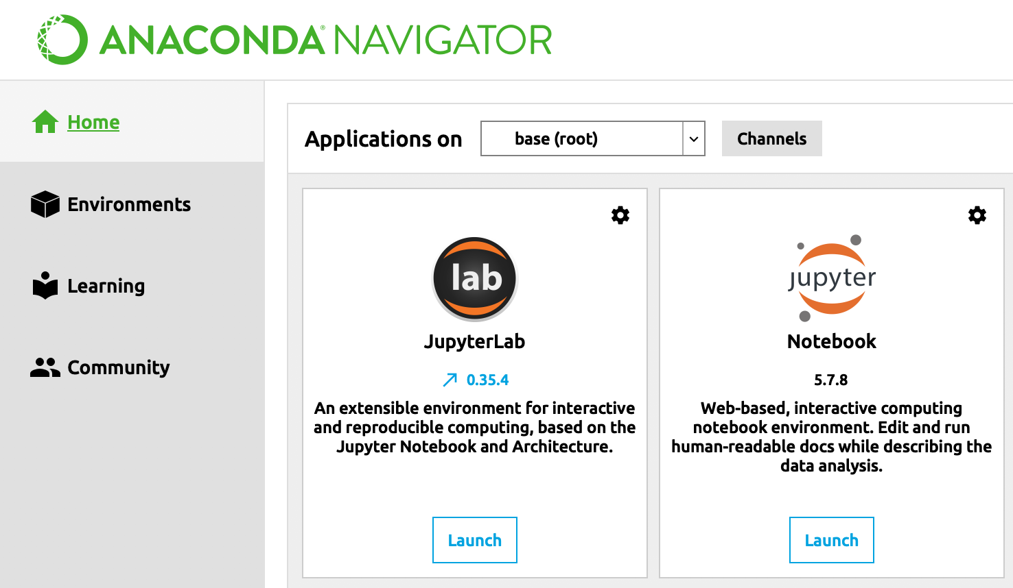
Anaconda Navigator interface
If you prefer to use the command line instead of Anaconda Navigator, once you have Anaconda installed, you should be able to open a new Terminal window (Mac) or Command Prompt (Win) and run jupyter notebook to launch the web browser with the Jupyter Notebook application. If you are using the command line to launch Jupyter Notebook, pay attention to the directory you are in when you launch it. That folder becomes the home directory that will appear immediately in the Jupyter Notebook interface, as described below.
Either approach will open up a new window or tab in your default browser with the Jupyter Notebook interface. Jupyter Notebook is browser-based: you only interact with it through your browser, even when Jupyter Notebook is running on your own computer.
Navigating the Jupyter Notebook interface
The Jupyter Notebook file browser interface is the main way to open a Jupyter notebook (.ipynb) file. If you try to open one in a plain text editor, the notebook will be displayed as a JSON file, not with interactive code blocks. To view a notebook through the Jupyter interface, you have to launch Jupyter Notebook first (which will display in a browser window), and open the file from within Jupyter Notebook. Unfortunately, there is no way to set Jupyter Notebook as the default software application to open .ipynb files when you double-click on them.
When you launch Jupyter Notebook from Anaconda Navigator, it automatically displays your home directory. This is usually the directory with your username on a Mac (/Users/your-user-name). On a PC it is usually C:\. If you launch Jupyter Notebook from the command line, it will display the contents of the folder you were in when you launched it. (Using the command line, you can also directly launch a specific notebook, e.g. jupyter notebook example.ipynb.)
To avoid cluttering this folder, you can make a new folder within this directory for your notebooks. You can either do this in your usual file management interface (Finder on Mac, or File Explorer on Windows), or within Jupyter Notebook itself, since Jupyter Notebook, much like Google Drive, provides a file management interface within a browser, as well as a menu-and-toolbar UI for authoring files. To add a new folder within Jupyter Notebook, click on New in the upper right, and choose Folder. This will create a new folder called “Untitled Folder”. To change the name, click the checkbox to the left of the “Untitled Folder”, then click on the “Rename” button that appears under the “Files” tab. Name the folder notebooks. Click on it to open that folder.
Uploading the example data
The example CSV file for this lesson is an extract from Harry Potter fan fiction metadata scraped from the Italian fanfic site https://efpfanfic.net, then cleaned using a combination of regular expressions and OpenRefine. The CSV has three columns: the rating of the story (similar to a movie rating), the date it was originally published, and the most recent date it was updated. The rating options are verde (green), giallo (yellow), arancione (orange), and rosso (red). The publication and updated dates are automatically created when the story is posted to the site or updated, so you can count on them being consistent.
Thanks to the consistency of the automatically-generated dates, it should be doable to convert them all into days of the week using Python. But if you don’t have a lot of experience with doing date conversions using Python, a Jupyter Notebook can provide a convenient interface for experimenting with different modules and approaches.
Download the sample CSV file.
Within the Jupyter Notebook file browser, you should be inside the notebooks directory you just created. Towards the upper right, click the “Upload” button and upload the sample CSV file. It will be easiest to access if it’s in the same directory as the Jupyter notebook that you’ll create in the next step in order to convert the dates.
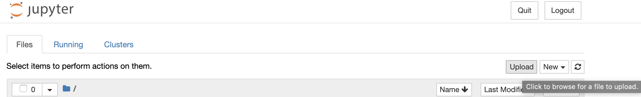
Uploading files in the Jupyter Notebook interface
Note that this isn’t the only way to make files appear in the Jupyter Notebook file browser. The notebooks folder you created is a regular directory on your computer, and so you can also use your usual file management interface (e.g. Finder on Mac, or File Explorer on Windows) to put .ipynb and/or data files in this directory. Jupyter notebooks use the location of the notebook file itself (the .ipynb file) as the default starting path. For workshops and courses, it may make sense to create a folder where you can store the notebook, any attached images, and the data you’re going to work with, all together. If everything isn’t in the same folder, you’ll have to include the path when referencing it, or use Python code within the notebook to change the working directory.
Creating a new notebook
Inside the notebooks folder, create a new Jupyter notebook to use to convert the dates for your research project. Click the “New” button in the upper right of the Jupyter Notebook file browser interface. If you’ve just installed Anaconda as described above, your only option will be to create a Jupyter notebook using the Python 3 kernel (the backend component that actually runs the code written in the notebook), but we’ll discuss below how to add kernels for other languages. Click on “Python 3”, and Jupyter Notebook will open a new tab with the interface for Jupyter notebooks themselves. By default, the notebook will be named “Untitled”; you can click on that text at the top of the screen to rename it.
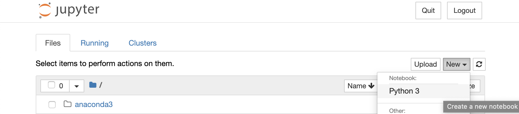
Creating a new Jupyter notebook
Working in Jupyter notebooks
A notebook is made up of cells: boxes that contain code or human-readable text. Every cell has a type, which can be selected from the drop-down options in the menu. The default option is “Code”; human-readable text boxes should use the “Markdown” type, and will need to be written using Markdown formatting conventions. To learn more about Markdown, see the “Getting Started With Markdown” Programming Historian lesson.
When you create a new Jupyter notebook, the first cell will be a code cell. At the top of the Jupyter Notebook interface is a toolbar with functions that apply to the currently-selected cell. One of the functions is a dropdown that reads “Code” by default. Click on this dropdown and select “Markdown”. (You can also use a keyboard shortcut, esc + m, to change the current cell to Markdown, and esc + y changes it back to a code cell.) We’ll start this notebook with a title and a brief explanation of what the notebook is doing. For the moment, this is just for your own memory and reference; you don’t want to invest too much in prose and formatting at this stage of the project, when you don’t know whether you’ll end up using this code as part of your final project, or if you’ll use a different tool or method. But it can still be helpful to include some markdown cells with notes to help you reconstruct your process.
Paste the following into the first cell. If it doesn’t appear with the first line in a large font (as a header), make sure you’ve selected “Markdown” from the dropdown at the top.
# Fanfic date conversion
Converting published & updated dates for Italian fanfic into days of the week.
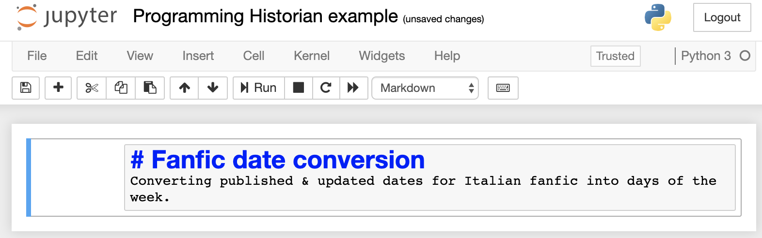
Editing Markdown cell in a Jupyter notebook
When you’re editing a cell, you can use Ctrl + Z (Win) or Command + Z (Mac) to undo changes that you’ve made. Each cell retains its own edit history; even if you move to a different cell and make edits there, you can subsequently click back on the first cell and undo your earlier changes there, without losing the changes to the second cell.
To leave editing mode and “run” this cell (for a Markdown cell, this doesn’t do anything, just moves you further down the notebook), you can click in the toolbar or press Ctrl+Enter (Ctrl+Return on Mac). If you want to resume editing it later, you can either double-click it, or select the cell (which will show a vertical blue line on the left once it’s selected) by clicking it once, and then hitting the Enter (Win) or Return (Mac) key. To leave editing mode, you can click in the toolbar or press Ctrl+Enter (Ctrl+Return on Mac). If you want to run your current cell and add a new cell (by default, a code cell) immediately below it, you can press Alt+Enter (Option+Enter on Mac).
Next, you need to figure out how to do the conversion. Searching for relevant terms may lead you to this StackOverflow discussion, and the first answer involves using the datetime Python module. As a first step, you need to import datetime, using a code cell. You also know that your input file is a CSV, so you should import the csv module as well.
To add a new cell, click the plus button in the toolbar (or use the esc + b keyboard shortcut). This will create a new code cell below the cell that’s currently selected. Create a new code cell, and paste in the following code to import a Python module:
import datetime
import csv
Thinking ahead to possibly sharing this notebook or some derivative, it may be useful to split out the module imports into one cell, and put the code itself into another cell, so that you can include a Markdown cell in between that explains what each one is doing.
Both of the packages that you’re importing into this notebook are already installed as part of Anaconda, but there are many niche packages relevant to research (e.g. the Classical Languages Toolkit, CLTK, for doing text analysis on historical languages) that aren’t included with Anaconda, and aren’t available through the conda installer. If you need a package like that, you have to install it using pip. Installing packages from within Jupyter notebooks can be a little tricky, because there may be differences between the Jupyter kernel that the notebook is using, and other versions of Python you may have installed on your computer. You can find a lengthy, technical discussion of the issues in this blog post.
If you are working on a notebook that you want to share, and it involves less-common packages, you can either include instructions in a Markdown cell that users should install the packages using conda or pip in advance, or you can use:
import sys
!conda install --yes --prefix {sys.prefix} YourModuleNameHere
to install something from the notebook using conda; the ! syntax indicates the code is executing something from the command line, rather than the Jupyter kernel. Or, if the package isn’t available in conda (many niche packages relevant for research aren’t), you can use pip:
import sys
!{sys.executable} -m pip install YourModuleNameHere
If you hadn’t installed Python on your computer prior to installing Anaconda for this lesson, you may need to add the pip package to be able to use it to install other packages. You can add it via the Anaconda Navigator GUI, or run conda install pip from the command line.
Returning to our example, next add another new code cell, and paste in the following code (making sure to include the tabs):
with open('ph-jupyter-notebook-example.csv') as f:
    csv_reader = csv.reader(f, delimiter=',')
    for row in csv_reader:
        datetime.datetime.strptime(row[1], '%d/%m/%Y').strftime('%A')
        print(row)
Clicking the button in the toolbar when you have a Code cell selected executes the code inside the cell. (If you try running this code after you’ve run the import statements, you’ll see an error: “ValueError: time data ‘1/7/18’ does not match format ‘%d/%m/%Y’”. Don’t worry – we’ll debug this next.)
After you run a code cell, a number will appear in brackets to the left of the cell. This number indicates the order in which the cell was run. If you go back and run the cell again, the number is updated.
If a number doesn’t immediately appear next to the cell, you’ll see an asterisk in brackets. This means that the code cell hasn’t finished running. This is common for computationally-intensive code (e.g. natural language processing) or long-running tasks like web scraping. Whenever a code cell is running, the favicon in the notebook’s browser tab changes to an hourglass . If you want to change tabs and do something else while the code is running, you can tell that it’s done when the hourglass changes back to the notebook icon .
Running a code cell in a Jupyter notebook
Run the two code cells in the notebook, starting from the top.
After you’ve run the second code cell, you’ll see an error. To figure out what’s happening, you can consult the documentation for datetime which explains each of the different formatting options. There, you’ll find that the only option for day values assumes zero-padded dates (i.e. single-digit days are prefixed with a 0). Looking at the example data, the months (listed second in this date order) are zero-padded, but not the days. You have two options: you can try to change the data, or you can try to change your code.
Let’s say that you want to try a different approach, but want to leave what you’ve done so far, in case you want to revisit that code, and maybe use it after changing the data. To help yourself remember what happened, add a Markdown cell above your second code cell. Click in the first code cell, then click the plus button in the toolbar. If you just click the plus button in the toolbar after running the last code cell, the new cell will appear at the bottom of the notebook. You can move it up to where you want it by clicking the up button. Make sure you’re in Markdown mode, and paste the following text:
### Doesn't work, needs zero-padded dates per [datetime documentation](https://docs.python.org/2/library/datetime.html?highlight=strftime#strftime-and-strptime-behavior). Modify source file?
Reading further in the StackOverflow discussion, there’s another approach that uses a different library, dateutil, that appears to be more flexible with the kinds of dates that it accepts. Go back up to the cell you used to import modules, and edit it to add (anywhere in that cell, as long as each import statement is on its own line):
import dateutil
Re-run that code cell; note that the number next to the cell changes the second time you run it.
Now create a new Markdown cell at the bottom of the notebook, and paste:
### trying dateutil for parsing dates, as per https://stackoverflow.com/a/16115575
Below it, add a new code cell with the following code (paying attention to the tabs, so that the code is indented just like you see it below):
with open('ph-jupyter-notebook-example.csv') as f:
    csv_reader = csv.reader(f, delimiter=',')
    for row in csv_reader:
        parseddate = dateutil.parser.parse(row[1])
        print(parseddate)
Run the cell with the code that you’ve just added. It may take longer; keep waiting until the asterisk next to the code cell turns into a number. The result should show the list of publication dates, formatted differently, with hyphen rather than slashes, and with the hours, minutes, seconds added (as zeroes, because the dates as recorded don’t include that data). At first glance, it seems like this worked, but if you compare it more closely with the source file, you’ll see that it’s not being consistent in how it parses the dates. Dates where the day value is greater than 12 are getting parsed correctly (it knows a value greater than 12 can’t be a month), but when the date value is 12 or less, the date is being parsed with the month first. The first line of the source file has the date 1/7/18, which gets parsed as “2018-01-07 00:00:00”. In the documentation for dateutil, you’ll find that you can specify dayfirst=true to fix this. Edit the last code cell, and change the second to last line to read:
parseddate = dateutil.parser.parse(row[1], dayfirst=True)
When you rerun the line, you’ll see that all the dates have been parsed correctly.
Parsing the date is just the first step – you still need to use the datetime module to convert the dates to days of the week.
Delete the last line of the code block, and replace it with the following (making sure you have the same level of indentation as the previous last line, for both of these lines):
        	dayofweek = datetime.date.strftime(parseddate, '%A')
        	print(dayofweek)
Rerun the code block. This should give you a list of days of the week.
Now that you have code to parse and reformat one date, you need to do it for both dates in each line of your source file. Because you know you have working code in the current code cell, if you’re not very comfortable with Python, you might want to copy the current code cell before you make modifications. Select the cell you want to copy and click the copy button in the toolbar; the paste button will paste the cell below whatever cell is currently selected. Making a copy allows you to freely make changes to the code, knowing that you can always easily get back to a version that works.
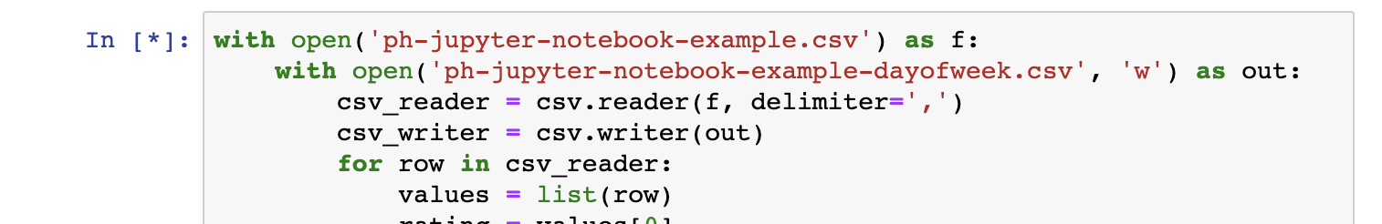
If you don’t want to work it out on your own, you can copy and paste this code into a new code cell or replace the current code cell:
#identifies the source file to open, calls it f
with open('ph-jupyter-notebook-example.csv') as f:
    #creates an output file (referred to as "out" in the notebook) for you to write to
    with open('ph-jupyter-notebook-example-dayofweek.csv', 'w') as out:
        #defines "csv_reader" as running the function csv.reader on the file
        csv_reader = csv.reader(f, delimiter=',')
        #defines "csv_writer" as running the functin csv.writer to "out" (the output file)
        csv_writer = csv.writer(out)
        #for each row that's being read by csv_reader...
        for row in csv_reader:
            #defines "csv_reader" as running the function csv.reader on the file
            csv_reader = csv.reader(f, delimiter=',')
            #for each row that's being read by csv_reader...
            for row in csv_reader:
            #creates a list called "values" with the contents of the row
              values = list(row)
              #defines "rating" as the first thing in the list
              #counting in Python starts with 0, not 1
              rating = values[0]
              #defines "parseddatepub" as the second thing (1, because we start with 0) in the list,
              #converted into a standard date format using dateutil.parser
              #and when those dates are parsed, the parser should know
              #that the first value in the sequence is the day
              parseddatepub = dateutil.parser.parse(values[1], dayfirst=True)
              #same as above for the updated date, the third thing (2) in the list
              parseddateupdate = dateutil.parser.parse(values[2], dayfirst=True)
              #defines "dayofweekpub" as parseddatepub (defined above), converted to the day of week
              #%A is what you use to change it to the day of the week
              #You can see othe formats here: https://docs.python.org/3/library/datetime.html#strftime-and-strptime-behavior
              dayofweekpub = datetime.date.strftime(parseddatepub, '%A')
              #same thing for update date
              dayofweekupdate = datetime.date.strftime(parseddateupdate, '%A')
              #creates a list of the rating and the newly formatted dates
              updatedvalues = [rating, dayofweekpub, dayofweekupdate]
              #writes all the values under this code cell
              csv_writer.writerow(updatedvalues)
              print(updatedvalues)
After you run this code, you will have a new file, ph-jupyter-notebook-example-dayofweek.csv, with your data in the format you need for analysis.
Now that you have working code to convert the dates from the form you have to the form you need, you can clean up the false starts and notes to yourself. You’ll want to keep the first code cell with the import statements, and the first Markdown cell with the title and description, but you should delete other Markdown and code cells that aren’t your final code. To delete a cell, click on it, then click the scissors button in the toolbar. If you delete a cell by mistake, you can click on Edit in the menu and choose “Undo Delete Cells”.
Saving, exporting, and publishing Jupyter notebooks
Jupyter autosaves your work periodically by creating “checkpoints”. If something goes wrong with your notebook, you can revert to a previous checkpoint by going to “File”, then “Revert to Checkpoint”, and choosing a timestamp. That said, it’s still important to save your notebook (using the save button ), because if you close and shut down the notebook kernel (including restarting the kernel), the checkpoints will be lost.
You can also download the notebook (File > Download as) in several different file formats. Downloading the Notebook format (.ipynb) is useful if you want to share your code in its full notebook format. You can also download it as code in whatever language your notebook is in (e.g. .r if in R or .py if Python or .js if JavaScript), as an .html file, as a markdown (.md) file, or as a PDF via LaTeX. If you download it as code, the Markdown cells become comments. (If you want to convert an .ipynb file to another format after you’ve downloaded it, you can use the nbconvert utility.)
If you’re working on a research project, you can use a Jupyter notebook, or a series of notebooks, along the way to keep track of your workflow. Some scholars post these notebooks on GitHub, along with slides or poster PDFs, and source data (or metadata, copyright permitting), to accompany presentations and talks. GitHub renders non-interactive versions of notebook files, so they can be previewed within a repo. Alternately, you can paste the URL of a GitHub repo that has Jupyter notebooks into nbviewer, which can sometimes a faster and more reliable preview. You may want to include a Markdown cell with a recommended citation for your Jupyter notebook, and a pointer to the GitHub repo where it is stored, especially if your notebook includes code that others might be able to reuse for similar analyses.
The code you just developed as part of this lesson belongs somewhere in the middle of a real project. If you’re using notebooks to document your workflow, you might choose to add the new code cell to an existing notebook, rather than downloading it as a separate, stand-alone notebook. Jupyter notebooks can be particularly helpful for documenting project workflows when you’re working with collaborators who may only be involved for a short period of time (such as summer undergraduate interns). With short-term collaborators, it’s important to help them understand and start using the project’s workflows without a lot of start-up time, and Jupyter notebooks can lay out these workflows step-by-step, explain where and how files are stored, and provide pointers to external tutorials and training materials to help collaborators who are less familiar with the project’s technical underpinnings get started. For instance, two projects that have used Jupyter notebooks to publish workflows are Sarah McEleney’s Socialist Realism Project and Mary Chester-Kadwell’s “text mining of English children’s literature 1789-1914 for the representation of insects and other creepy crawlies”.
As your project progresses, if you’re publishing through open-access channels, and your data sets can be freely redistributed, Jupyter notebooks can provide an ideal format for making the code underpinning your scholarly argument visible, testable, and reusable. While journals and presses may not accept Jupyter notebooks as a submission format, you could develop a notebook “version” of your paper that includes the full text (as Markdown cells), with code cells integrated into the flow of the scholarly narrative as an immediately accessable illustration of the analysis you’re describing. You could also include the code cells that make up the data preparation workflows as an appendix, either in the same notebook, or in a separate one. Integrating the code with the text of a scholarly article makes it far more likely that readers will actually engage with the code, since they can simply run it within the same notebook where they’re reading the argument. Some scholars, particularly in Europe, also post their notebooks to Zenodo, an archive for research regardless of the country of origin, funder, or discipline. Zenodo supports data sets up to 50 GB (vs. the 100 MB file size limit on Github), and provides DOIs for uploaded material, including notebooks. Some scholars combine archiving on Zenodo for sustainability with publishing on GitHub for findability, by including the Zenodo DOI as part of the readme.md file in the GitHub repository that includes the notebooks. As an example, Giovanni Colavizza and Matteo Romanello’s “Applied Data Analytics” workshop notebook for DHOxSS 2019 is published on GitHub but includes a Zenodo DOI.
While fully integrated argumentation and code are still hard to find due to the lack of a venue for publishing this kind of work, scholars have started using Jupyter notebooks as a more interactive incremental steps towards dynamic computational publications. José Calvo has an example of a notebook accompanying an article on stylometry (in Spanish), and Jed Dobson published a set of notebooks to accompany his book Critical Digital Humanities: The Search for a Methodology, which directly addresses Jupyter notebooks as scholarly objects (p. 39-41).
Using Jupyter notebooks for teaching
Jupyter Notebooks are a great tool for teaching coding, or for teaching concepts such as topic modeling or word vectors that involve coding. The ability to provide instructions and explanations as Markdown allows for educators to give detailed notes on the code through alternating Markdown and code cells, so that the Markdown text explains the code in the cell just below. This is helpful for hands-on workshops, as the instructions and code can be written in advance. This enables attendees to just open the notebook, download a dataset, and run the code as-is. If you expect to teach a workshop where students will have different levels of familiarity with coding, you can set up the notebook to have supplemental tasks for the students who are comfortable modifying code. At the same time, even the students who are hesitant about touching the code will still be able to achieve the main outcome of the workshop just by running pre-written code cells.
As another approach, you can also use Jupyter notebooks for writing code as you go. In such a workshop, students can start with a blank notebook, and and write the code along with you. The cells help segment the code as you write it, as opposed to using a text editor or IDE (Integrated Development Environment) which does not break up the code as neatly and can cause confusion, especially when teaching beginners.
You can use Jupyter notebooks for classroom assignments by giving directions in Markdown and having students write code in a blank cell based on the instructions. In this way, you can create an interactive coding assignment that teaches students not only the syntax and vocabulary of a coding language, but can also explain the best practices of coding in general.
If you’re already using Jupyter notebooks for documenting the workflow for your project, you may be able to reframe these research notebooks for classroom use, as one way of bringing your research into the classroom. This example pedagogical notebook is a hybrid of some of the pedagogical approaches described above. The first section of the notebook is intended for students who have little or no previous experience running code; the major learning outcome is to compare the time it takes to manually convert data formats, compared to doing it with code. You could use this notebook for a hands-on lab session in an intro to digital humanities or digital history, where all the students install Anaconda and learn the basics of Jupyter notebooks. If the class has a mix of students with no technical background and students with previous exposure to Python, you could direct the students with programming experience to work together in groups of two or three to propose solutions to the prompts in the second part of the notebook. Keep in mind that if you use a class assignment like this as a way to have computer science students write code that helps your research project, they should be credited as collaborators and acknowledged in subsequent publications coming from the project4.
There are many digital humanities “Intro to Python” courses and workshops that use Jupyter notebooks (including Introduction à Python et au développement web avec Python pour les sciences humaines by Thibault Clérice, translated from material by Matthew Munson). Jupyter notebooks are also commonly used in text analysis workshops, such as the word vectors workshop at DH 2018, taught by Eun Seo Jo, Javier de la Rosa, and Scott Bailey.
Teaching with Jupyter notebooks doesn’t always have to involve the time-consuming process of downloading and installing Anaconda, especially if you’re envisioning only having one or two lessons that involve notebooks. If your classroom activities with Jupyter notebooks involve using example data that you’ve already prepared, and if you’ve already written at least some of the code, you may want to explore running Jupyter notebooks using free cloud computing resources, as long as your students are guaranteed to have reliable internet connectivity in the classroom. Running notebooks in the cloud also provides a consistent environment for all students, sparing you from having to negotiate differences between Windows and Mac, or provide an alternative for students whose laptops lack the hard drive space or memory to run Anaconda effectively.
Because the options are evolving quickly, it’s best to use your favorite search engine to find a recent list of cloud computing options for Jupyter Notebooks. One project that has seen particular uptake among academic users of notebooks is MyBinder, which will take a GitHub repository that contains Jupyter notebook .ipynb files related data (embedded images, data sets you want to use the notebooks on, etc.), and information about necessary packages and dependencies (in a requirements.txt or environment.yml file), and make it launchable using a cloud server. Once you’ve had MyBinder package up your GitHub repo, you can add a Binder “badge” to the readme file for the repo. Anyone viewing the repo can launch the notebook directly from their browser, without having to download or install anything.
Because the data that the notebook needs to access has to be included in the repo, this won’t work for all situations (e.g. if the data can’t be legally redistributed on GitHub, exceeds GitHub’s maximum file size and can’t be downloaded from elsewhere as part of the Binder environment setup, or if you want people to use the notebook with their own data), but it’s a great option for workshops or classes where everyone is working with the same, shareable data.
If you want to start exploring cloud options, Shawn Graham has created some templates for setting up Python and R Jupyter notebooks for use on Binder.
Finally, if you need to keep your notebooks out of the cloud (e.g. due to sensitive or otherwise restricted data) but want to provide a consistent environment for all your students, you can explore JupyterHub, which is has been adopted as core technical infrastructure for a growing number of data science programs.
Converting existing Python code
Even if you like the idea of using Jupyter Notebooks, any format conversion requires additional work. If you already have your code written as Python scripts, conversion to Jupyter Notebooks is fairly straightforward. You can copy and paste the code from your .py file into a single code cell of a new notebook, and then split the code cell into segments and add additional Markdown cells as needed.
Alternately, it may be easier to segment as you transfer the code, copying one segment at a time into a new code cell. Either method works and is a matter of personal preference.
There are also tools like the p2j package that automatically convert existing Python code to Jupyter notebooks, following a documented set of conventions (e.g. turning comments into Markdown cells).
Jupyter Notebooks for other programming languages
Jupyter Notebooks allow you to use many different programming languages including R, Julia, JavaScript, PHP, or Ruby. A current list of available languages can be found on the Jupyter Kernels GitHub page.
While Python is supported by default when you install Jupyter Notebook through Anaconda, the other programming languages need to have their language kernels installed before they can be run in Jupyter Notebook. The installation instructions are different for each language kernel, so it is best to just find and follow the instructions for your preferred language. At least for R, this is relatively straightforward. The Jupyter Kernels GitHub page has links to instructions for all available language kernels.
Once you have the kernel for your desired language(s) installed, you can run notebooks written in that programming language, or you can create your own notebooks that execute that language. Each language with a kernel installed on your computer will be available as an option when you create a new notebook as described above.
As an example of an R notebook, see this Jupyter adaptation of Andrew Piper’s R code from “Enumerations”.
Scaling up computation with Jupyter notebooks
Especially if you’re new to writing Python, just getting anything to work can feel like a victory. If you start working with bigger data sets, though, you may discover that some of the initial “solutions” you found (such as using .readlines() for reading a text file line by line) turn out to be computationally inefficient, to the point of causing problems. One way of starting to understand inefficiencies in your code is to add %%timeit to the top of a cell. The notebook will choose a number of iterations to run the code, depending on the complexity of the task, and will print the number of iterations and the average time. Doing multiple iterations, rather than just one, can be helpful to account for small system-level delays (e.g. if your laptop is momentarily bogged down with other processes.) If you want to time multiple iterations of a single line, rather than the whole cell, you can put %timeit in front of the line. Be careful with how you apply these: sorting a list will take much longer for the first iteration than the second, after the list is already in order. In cases like list sorting where it doesn’t make sense to measure multiple iterations, or for long-running tasks where small system-level delays won’t have a significant impact, you can use %%time at the top of a cell, or %time in front of a line, which measures the time a single run takes. These commands are part of a family of built-in “magic commands” available in Jupyter notebooks; see the Jupyter documentation for more details.
Getting some sense for how long your code is likely to run is an important prerequisite for scaling up to larger compute resources, like the centrally-funded high performance computing (HPC) clusters available at many institutions. An overwhelming majority of the researchers who use these resources are in the sciences, but usually any faculty member can request access. You may also be able to get access to regional or national HPC resources. These compute resources can significantly speed up large compute jobs, especially tasks like 3D modeling that can take advantage of compute nodes with powerful graphics processing units (GPUs). Learning how to use HPC clusters is a topic large enough for its own lesson, but Jupyter notebooks may enable you to take a shortcut. Some research computing groups offer easier ways for researchers to run Jupyter Notebooks using HPC cluster resources, and you can find multiple general-purpose guides and examples for doing it. If you can get access to HPC resources, it’s worth reaching out to the research computing IT staff and inquiring about how you can run your Jupyter notebooks on the cluster, if you don’t see documentation on their website. Research IT staff who work primarily with scientists may communicate more brusquely than you’re accustomed to, but don’t let it turn you off – most research IT groups are enthusiastic about humanists using their resources and want to help, because disciplinary diversity among their user base is important for their metrics at the university level.
Conclusion
From experimenting with code to documenting workflows, from pedagogy to scholarly publication, Jupyter notebooks are a flexible, multi-purpose tool that can support digital research in many different contexts. Even if you aren’t sure how exactly you’ll use them, it’s fairly easy to install the Jupyter Notebook software and download and explore existing notebooks, or experiment with a few of your own. Jupyter notebooks hold a great deal of promise for bridging the critical and computational facets of digital humanities research. To conclude with a quote from Jed Dobson’s Critical Digital Humanities: The Search for a Methodology:
Notebooks are theory — not merely code as theory but theory as thoughtful engagement with the theoretical work and implications of the code itself. Disciplinary norms— including contextual framing, theory, and self or auto-critique— need to accompany, supplement, and inform any computational criticism. Revealing as much of the code, data, and methods as possible is essential to enable the ongoing disciplinary conversation. Compiling these together in a single object, one that can be exported, shared, examined, and executed by others, produces a dynamic type of theorization that is modular yet tightly bound up with its object.5
Links
- A growing list of Jupyter notebooks for DH, in multiple human and programming languages. Thanks to everyone who sent suggestions on Twitter; additional references are welcome.
- A detailed technical description of installing Python packages from Jupyter.
Acknowledgements
-
Thanks to Stéfan Sinclair for the references to previous discussions of notebook usage in digital humanities.
-
Thanks to Rachel Midura for suggesting the use of Jupyter notebooks for collaboration.
-
Thanks to Paige Morgan for the reminder about the importance of emphasizing state issues.
-
Knuth, Donald. 1992. Literate Programming. Stanford, California: Center for the Study of Language and Information. ↩
-
Millman, KJ and Fernando Perez. 2014. “Developing open source scientific practice”. In Implementing Reproducible Research, Ed. Victoria Stodden, Friedrich Leisch, and Roger D. Peng. https://osf.io/h9gsd/ ↩
-
Sinclair, Stéfan & Geoffrey Rockwell. 2013. “Voyant Notebooks: Literate Programming and Programming Literacy”. Journal of Digital Humanities, Vol. 2, No. 3 Summer 2013. http://journalofdigitalhumanities.org/2-3/voyant-notebooks-literate-programming-and-programming-literacy/ ↩
-
Haley Di Pressi, Stephanie Gorman, Miriam Posner, Raphael Sasayama, and Tori Schmitt, with contributions from Roderic Crooks, Megan Driscoll, Amy Earhart, Spencer Keralis, Tiffany Naiman, and Todd Presner. “A Student Collaborator’s Bill of Rights”. https://humtech.ucla.edu/news/a-student-collaborators-bill-of-rights/ ↩
-
Dobson, James. 2019. Critical Digital Humanities: The Search for a Methodology. Urbana-Champaign: University of Illinois Press. p. 40. ↩
