Contents
- Lesson goals
- Why should historians care about data quality?
- Description of the tool: OpenRefine
- Description of the exercise: Powerhouse Museum
- Conclusions
Lesson goals
Don’t take your data at face value. That is the key message of this tutorial which focuses on how scholars can diagnose and act upon the accuracy of data. In this lesson, you will learn the principles and practice of data cleaning, as well as how OpenRefine can be used to perform four essential tasks that will help you to clean your data:
- Remove duplicate records
- Separate multiple values contained in the same field
- Analyse the distribution of values throughout a data set
- Group together different representations of the same reality
These steps are illustrated with the help of a series of exercises based on a collection of metadata from the Powerhouse museum, demonstrating how (semi-)automated methods can help you correct the errors in your data.
Why should historians care about data quality?
Duplicate records, empty values and inconsistent formats are phenomena we should be prepared to deal with when using historical data sets. This lesson will teach you how to discover inconsistencies in data contained within a spreadsheet or a database. As we increasingly share, aggregate and reuse data on the web, historians will need to respond to data quality issues which inevitably pop up. Using a program called OpenRefine, you will be able to easily identify systematic errors such as blank cells, duplicates, spelling inconsistencies, etc. OpenRefine not only allows you to quickly diagnose the accuracy of your data, but also to act upon certain errors in an automated manner.
Description of the tool: OpenRefine
In the past, historians had to rely on information technology specialists to diagnose data quality and to run cleaning tasks. This required custom computer programs when working with sizeable data sets. Luckily, the advent of Interactive Data Transformation tools (IDTs) now allows for rapid and inexpensive operations on large amounts of data, even by professionals lacking in-depth technical skills.
IDTs resemble the desktop spreadsheet software we are all familiar with, and they share some common functionalities. You can for example use an application such as Microsoft Excel to sort your data based on numerical, alphabetical and custom-developed filters, which allows you to detect errors more easily. Setting up these filters in a spreadsheet can be cumbersome, as they are a secondary functionality. On a more general level, we could say that spreadsheets are designed to work on individual rows and cells, whereas IDTs operate on large ranges of data at once. These ‘spreadsheets on steroids’ offer an integrated and user-friendly interface through which end users can detect and correct errors.
Several general purpose tools for interactive data transformation have been developed in recent years, such as Potter’s Wheel ABC and Wrangler. Here we want to focus specifically on OpenRefine (formerly Freebase Gridworks and Google Refine), as in the opinion of the authors, it is the most user-friendly tool to efficiently process and clean large amounts of data in a browser-based interface.
On top of data profiling and cleaning operations, OpenRefine extensions allow users to identify concepts in unstructured text, a process referred to as named-entity recognition (NER), and can also reconcile their own data with existing knowledge bases. By doing so, OpenRefine can be a practical tool to link data with concepts and authorities which have already been declared on the Web by parties such as Library of Congress or OCLC. Data cleaning is a prerequisite to these steps; the success rate of NER and a fruitful matching process between your data and external authorities depends on your ability to make your data as coherent as possible.
Description of the exercise: Powerhouse Museum
The Powerhouse Museum in Sydney provided a metadata export of its collection on its website. The museum is one of the largest science and technology museums worldwide, providing access to almost 90,000 objects, ranging from steam engines to fine glassware and from haute couture to computer chips.
The Powerhouse actively disclosed its collection online and made most of its data freely available. From the museum website, a tab-separated text file under the name phm-collection.tsv could be downloaded, and opened as a spreadsheet. The unzipped file (58MB) contains basic metadata (17 fields) for 75,823 objects, released under a Creative Commons Attribution Share Alike (CCASA) license. In this tutorial we will be using a copy of the data that we have archived for you to download (in a moment). This ensures that if the Powerhouse Museum updates the data, you will still be able to follow along with the Lesson.
Throughout the data profiling and cleaning process, the case study will
specifically focus on the Categories field, which is populated with
terms from the Powerhouse museum Object Names Thesaurus (PONT). PONT
recognizes Australian usage and spelling, and reflects in a very direct
manner the strengths of the collection. In the collection you will find
better representations of social history and decorative arts, and
comparably few object names relating to fine arts and natural history.
The terms in the Categories field comprise what we call a Controlled vocabulary. A controlled vocabulary consists of keywords describing the content of a collection using a limited number of terms, and is often a key entry point into data sets used by historians in libraries, archives and museums. That is why we will give particular attention to the ‘Categories’ field. Once the data has been cleaned, it should be possible to reuse the terms in the controlled vocabulary to find additional information about the terms elsewhere online, which is known as creating Linked Data.
Getting started: installing OpenRefine and importing data
Download OpenRefine and follow the installation instructions. OpenRefine works on all platforms: Windows, Mac, and Linux. OpenRefine will open in your browser, but it is important to realise that the application is run locally and that your data won’t be stored online. The data files are archived on the Programming Historian site as phm-collection. Please download the phm-collection.tsv file before continuing.
On the OpenRefine start page, create a new project using the downloaded data file and click Next. By default, the first line will be correctly parsed as the name of a column, but you need to unselect the ‘Quotation marks are used to enclose cells containing column separators’ checkbox, since the quotes inside the file do not have any meaning to OpenRefine. Additionally, select the ‘Attempt to parse cell text into numbers’ checkbox to let OpenRefine automatically detect numbers. Now click on ‘Create project’. If all goes well, you will see 75,814 rows.
The Powerhouse museum data set consists of detailed metadata on all the collection objects, including title, description, several categories the item belongs to, provenance information, and a persistent link to the object on the museum website. To get an idea of what object the metadata corresponds to, simply click the persistent link and the website will open.
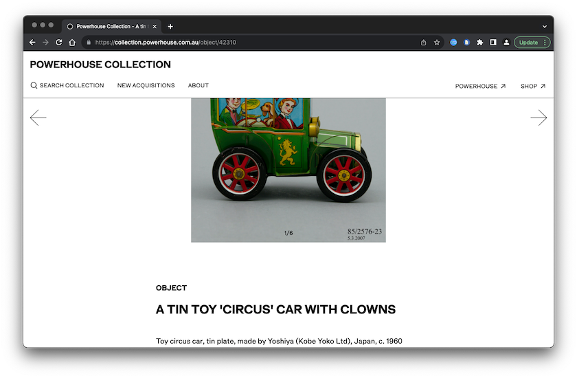
Figure 1: Screenshot of a Sample Object on the Powerhouse Museum Website
Get to know your data
The first thing to do is to look around and get to know your data. You
can inspect the different data values by displaying them in facets. You
could consider a facet like a lense through which you view a
specific subset of the data, based on a criterion of your choice. Click
the triangle in front of the column name, select Facet, and create a
facet. For instance, try a Text facet or a Numeric facet, depending
on the nature of the values contained in the fields (numeric values are
in green). Be warned, however, that text facets are best used on fields
with redundant values (Categories for instance); if you run into a ‘too
many to display’ error, you can choose to raise the choice count limit
above the 2,000 default, but too high a limit can slow down the
application (5,000 is usually a safe choice). Numeric facets do not have
this restriction. For more options, select Customized facets: facet by
blank, for instance, comes handy to find out how many values were filled
in for each field. We’ll explore these further in the following
exercises.
Remove blank rows
One thing you notice when creating a numeric facet for the Record ID column, is that three rows are empty. You can find them by unselecting the Numeric checkbox, leaving only Non-numeric values. Actually, these values are not really blank but contain a single whitespace character, which can be seen by moving your cursor to where the value should have been and clicking the ‘edit’ button that appears. To remove these rows, click the triangle in front of the first column called ‘All’, select ‘Edit rows’, and then ‘Remove all matching rows’. Close the numeric facet to see the remaining 75,811 rows.
Removing duplicates
A second step is to detect and remove duplicates. These can be spotted by sorting them by a unique value, such as the Record ID (in this case we are assuming the Record ID should in fact be unique for each entry). The operation can be performed by clicking the triangle left of Record ID, then choosing ‘Sort‘… and selecting the ‘numbers’ bullet. In OpenRefine, sorting is only a visual aid, unless you make the reordering permanent. To do this, click the Sort menu that has just appeared at the top and choose ‘Reorder rows permanently’. If you forget to do this, you will get unpredictable results later in this tutorial.
Identical rows are now adjacent to each other. Next, blank the Record ID of rows that have the same Record ID as the row above them, marking them duplicates. To do this, click on the Record ID triangle, choose Edit cells > Blank down. The status message tells you that 84 columns were affected (if you forgot to reorder rows permanently, you will get only 19; if so, undo the blank down operation in the ‘Undo/Redo’ tab and go back to the previous paragraph to make sure that rows are reordered and not simply sorted). Eliminate those rows by creating a facet on ‘blank cells’ in the Record ID column (‘Facet’ > ‘Customized facets’ > ‘Facet by blank’), selecting the 84 blank rows by clicking on ‘true’, and removing them using the ‘All’ triangle (‘Edit rows’ > ‘Remove all matching rows’). Upon closing the facet, you see 75,727 unique rows.
Be aware that special caution is needed when eliminating duplicates. In the above mentioned step, we assume the dataset has a field with unique values, indicating that the entire row represents a duplicate. This is not necessarily the case, and great caution should be taken to manually verify whether the entire row represents a duplicate or not.
Atomization
Once the duplicate records have been removed, we can have a closer look at the Categories field. On average each object has been attributed 2.25 categories. These categories are contained within the same field, separated by a pipe character ‘|’. Record 9, for instance, contains three: ‘Mineral samples|Specimens|Mineral Samples-Geological’. In order to analyze in detail the use of the keywords, the values of the Categories field need to be split up into individual cells on the basis of the pipe character , expanding the 75,727 records into 170,167 rows. Choose ‘Edit cells’, ‘Split multi-valued cells’, entering ‘|’ as the value separator. OpenRefine informs you that you now have 170,167 rows.
It is important to fully understand the rows/records paradigm. Make the Record ID column visible to see what is going on. You can switch between ‘rows’ and ‘records’ view by clicking on the so-labelled links just above the column headers. In the ‘rows view’, each row represents a couple of Record IDs and a single Category, enabling manipulation of each one individually. The ‘records view’ has an entry for each Record ID, which can have different categories on different rows (grouped together in grey or white), but each record is manipulated as a whole. Concretely, there now are 170,167 category assignments (rows), spread over 75,736 collection items (records). You maybe noticed that we are 9 records up from the original 75,727, but don’t worry about that for the time being, we will come back to this small difference later.
Facetting and clustering
Once the content of a field has been properly atomized, filters, facets,
and clusters can be applied to give a quick and straightforward overview
of classic metadata issues. By applying the customized facet ‘Facet by
blank’, one can immediately identify the 461 records that do not have a
category, representing 0.6% of the collection. Applying a text facet to
the Categories field allows an overview of the 4,934 different
categories used in the collection (the default limit being 2,000, you
can click ‘Set choice count limit’ to raise it to 5,000). The headings
can be sorted alphabetically or by frequency (‘count’), giving a list of
the most used terms to index the collection. The top three headings are
‘Numismatics’ (8,041), ‘Ceramics’ (7,390) and ‘Clothing and dress’
(7,279).
After the application of a facet, OpenRefine proposes to cluster facet choices together based on various similarity methods. As Figure 2 illustrates, the clustering allows you to solve issues regarding case inconsistencies, incoherent use of either the singular or plural form, and simple spelling mistakes. OpenRefine presents the related values and proposes a merge into the most recurrent value. Select values you wish to cluster by selecting their boxes individually or by clicking ‘Select all’ at the bottom, then chose ‘Merge Selected and Re-Cluster’.
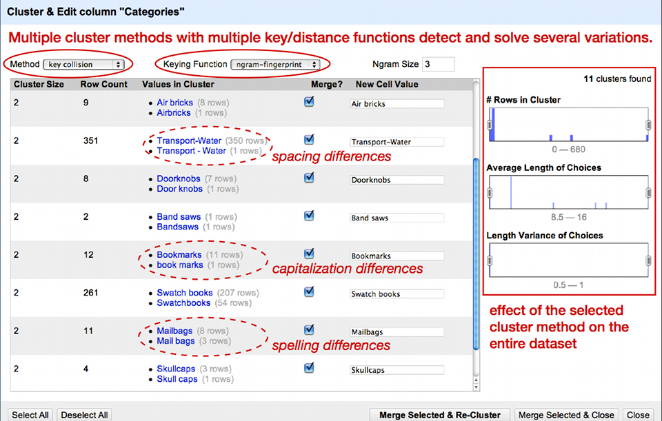
Figure 2 : Overview of some clusters
The default clustering method is not too complicated, so it does not find all clusters yet. Experiment with different methods to see what results they yield. Be careful though: some methods are too aggressive, so you might end up clustering values that do not belong together. Now that the values have been clustered individually, we can put them back together in a single cell. Click the Categories triangle and choose Edit cells, Join multi-valued cells, OK. Choose the pipe character (|) as a separator. The rows now look like before, with a multi-valued Categories field.
Applying ad-hoc transformations through the use of GREL expressions
You may remember there was an increase in the number of records after the splitting process: nine records appeared out of nowhere. In order to find the cause of this disparity, we need to go back in time before we split the categories into separate rows. To do so, toggle the Undo/Redo tab right of the Facet/Filter tab, and you will get a history of all the actions that you performed since the project was created. Select the step just before ‘Split multi-valued cells in column Categories’ (if you followed our example this should be ‘Remove 84 rows’) then go back to the Facet/Filter tab.
The issue arose during the splitting operation on the pipe character, so
there is a strong chance that whatever went wrong is linked to this
character. Let’s apply a filter on the Categories column by selecting
‘Text filter’ in the menu. First type a single | in the field on the
left: OpenRefine informs you that there are 71,064 matching records
(i.e. records containing a pipe) out of a total of 75,727. Cells that do
not contain a pipe can be blank ones, but also cells containing a single
category with no separator, such as record 29 which only has ‘Scientific
instruments’.
Now enter a second | after the first one to get || (double pipe): you
can see that 9 records are matching this pattern. These are likely the 9
records guilty of our discrepancy: when OpenRefine splits these up,
the double pipe is interpreted as a break between two records instead of
a meaningless double separator. Now how do we correct these values? Go
to the menu of the ‘Categories’ field, and choose ‘Edit cells’ >
‘Transform‘…. Welcome to the custom text tranform interface, a powerful
functionality of OpenRefine using the OpenRefine Expression Language
(GREL).
The word ‘value’ in the text field represents the current value of each cell, which you can see below. We can modify this value by applying functions to it (see the GREL documentation for a full list). In this case, we want to replace double pipes with a single pipe. This can be achieved by entering the following GREL expression (be sure not to forget the quotes):
value.replace('||', '|')
Under the ‘Expression’ text field, you get a preview of the modified values, with double pipes removed. Click OK and try again to split the categories with ‘Edit cells’ > ‘Split multi-valued cells’, the number of records will now stay at 75,727 (click the ‘records’ link to double-check).
* * *
Another issue that can be solved with the help of GREL is the problem
of records for which the same category is listed twice. Take record 41
for instance, whose categories are ‘Models|Botanical specimens|Botanical
Specimens|Didactic Displays|Models’. The category ‘Models’ appears twice
without any good reason, so we want to remove this duplicate. Click the
Categories triangle and choose Edit cells, Join multi-valued cells, OK.
Choose the pipe character as a separator. Now the categories are listed
as before. Then select ‘Edit cells’ > ‘Transform’, also on the
categories column. Using GREL we can successively split the categories
on the pipe character, look for unique categories and join them back
again. To achieve this, just type the following expression:
value.split('|').uniques().join('|')
You will notice that 33,008 cells are affected, more than half the collection.
Exporting your cleaned data
Since you first loaded your data into OpenRefine, all cleaning operations have been performed in the software memory, leaving your original data set untouched. If you want to save the data that you have been cleaning, you need to export them by clicking on the ‘Export’ menu top-right of the screen. OpenRefine supports a large variety of formats, such as CSV, HTML or Excel: select whatever suits you best or add your own export template by clicking ‘Templating’. You can also export your project in the internal OpenRefine format in order to share it with others.
Building on top of your cleaned data
Once your data has been cleaned, you can take the next step and explore other exciting features of OpenRefine. The user community of OpenRefine has developed two particularly interesting extensions which allow you to link your data to data that has already been published on the Web. The RDF Transform extension transforms plaintext keywords into URLs. The NER extension allows you to apply named-entity recognition (NER), which identifies keywords in flowing text and gives them a URL.
Conclusions
If you only remember on thing from this lesson, it should be this: all data is dirty, but you can do something about it. As we have shown here, there is already a lot you can do yourself to increase data quality significantly. First of all, you have learned how you can get a quick overview of how many empty values your dataset contains and how often a particular value (e.g. a keyword) is used throughout a collection. This lessons also demonstrated how to solve recurrent issues such as duplicates and spelling inconsistencies in an automated manner with the help of OpenRefine. Don’t hesitate to experiment with the cleaning features, as you’re performing these steps on a copy of your data set, and OpenRefine allows you to trace back all of your steps in the case you have made an error.