Contents
Overview
What if you only wanted to look at the pictures in a book? This is a thought that has occurred to young children and adult researchers alike. If you knew that the book was available through a digital library, it would be nice to download only those pages with pictures and ignore the rest.
Here are the page thumbnails for a HathiTrust volume with unique identifier osu.32435078698222. After the process described in this lesson, only those pages with pictures (31 in total) have been downloaded as JPEGs to a folder.
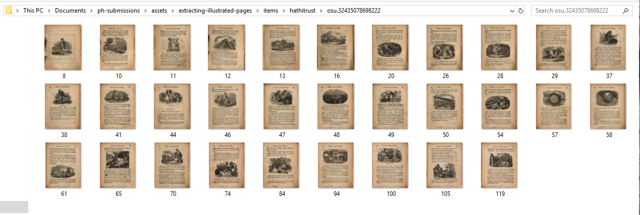
View of volume for which only pages with pictures have been downloaded.
To see how many unillustrated pages have been filtered out, compare against the full set of thumbnails for all 148 pages in this revised 1845 edition of Samuel Griswold Goodrich’s bestselling children’s book Tales of Peter Parley about America (1827).
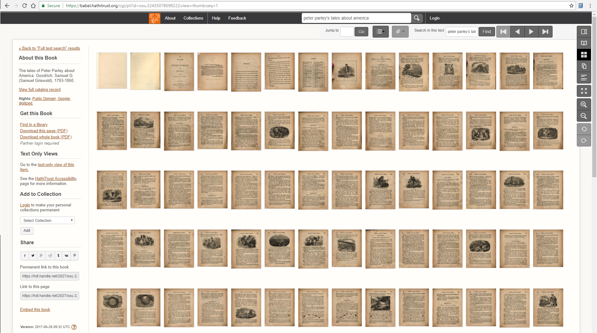
View of HathiTrust thumbnails for all pages.
This lesson shows how complete these filtering and downloading steps for public-domain text volumes held by HathiTrust (HT) and Internet Archive (IA), two of the largest digital libraries in the world. It will be of interest to anyone who wants to create image corpora in order to learn about the history of illustration and the layout (mise en page) of books. Visual approaches to digital bibliography are becoming popular, following the pioneering efforts of EBBA and AIDA. Recently completed or funded projects explore ways to identify footnotes and track marginalia, to give just two examples.
My own research tries to answer empirical questions about changes in the frequency and mode of illustration in nineteenth-century medical and educational texts. This involves aggregating counts of pictures per book and trying to estimate what printing process was used to make those pictures. A more targeted use case for extracting picture pages might be the collation of illustrations across different editions of the same book. Future work might profitably investigate the visual characteristics and meaning of the extracted pictures: their color, size, theme, genre, number of figures, and so on.
How to get localized information about visual regions of interest is beyond the scope of this lesson since the process involves quite a bit of machine learning. However, the yes/no classification of pages with (or without) pictures is a practical first step to shrink the huge space of all pages for each book in a target collection and, thereby making illustration localization feasible. To give a reference point, nineteenth-century medical texts contain (on average) illustrations on 1-3% of their pages. If you are trying to study illustration within a digital-library corpus about which you do not have any preexisting information, it is thus reasonable to assume that 90+% of the pages in that corpus will NOT be illustrated.
HT and IA allow the pictures/no pictures question to be answered indirectly through parsing the data generated by optical character recognition software (OCR is applied after a physical volume is scanned in order to generate an often-noisy transcription of the text). Leveraging OCR output to find illustrated pages was first proposed by Kalev Leetaru in a 2014 collaboration with Internet Archive and Flickr. This lesson ports Leetaru’s approach to HathiTrust and takes advantage of faster XML-processing libraries in Python as well as IA’s newly-extended range of image file formats.
Since HT and IA expose their OCR-derived information in slightly different ways, I will postpone the details of each library’s “visual features” to their respective sections.
Goals
By the end of the lesson you will be able to:
- Set up the “minimal” Anaconda Python distribution (Miniconda) and create an environment
- Save and iterate over a list of HT or IA volumes IDs generated by a search
- Access the HT and IA data application programmer interfaces (APIs) through Python libraries
- Find page-level visual features
- Download page JPEGs programmatically
The big-picture goal is to strengthen data collection and exploration skills by creating a historical illustration corpus. Combining image data with volume metadata allows the formulation of promising research questions about visual change over time.
Requirements
This lesson’s software requirements are minimal: access to a machine running a standard operating system and a web browser. Miniconda is available in both 32- and 64-bit versions for Windows, macOS, and Linux. Python 3 is the current stable release of the language and will be supported indefinitely.
This tutorial assumes basic knowledge of the command line and the Python programming language. You should understand the conventions for comments and commands in a shell-based tutorial. I recommend Ian Milligan and James Baker’s Introduction to the Bash Command Line for learning or brushing up on your command line skills.
Setup
Dependencies
More experienced readers may wish to simply install the dependencies and run the notebooks in their environment of choice. Further information on my own Miniconda setup (and some Windows/*nix differences) is provided.
hathitrust-api(Install docs)internetarchive(Install docs)jupyter(Install docs)requests(Install docs) [creator recommendspipenvinstallation; forpipinstall see PyPI]
Lesson Files
Download this compressed folder that contains two Jupyter notebooks, one for each of the digital libraries. The folder also contains a sample JSON metadata file describing a HathiTrust collection. Unzip and check that the following files are present: 554050894-1535834127.json, hathitrust.ipynb, internetarchive.ipynb.
Download Destination
Here is the default directory that will be created once all the cells in both notebooks have been run (as provided). After getting a list of which pages in a volume contain pictures, the HT and IA download functions request those pages as JPEGs (named by page number) and store them in sub-directories (named by item ID). You can of course use different volume lists or change the out_dir destination to something other than items.
items/
├── hathitrust
│   ├── hvd.32044021161005
│   │   ├── 103.jpg
│   │   └── ...
│   └── osu.32435078698222
│       ├── 100.jpg
│       ├── ...
└── internetarchive
    └── talespeterparle00goodgoog
        ├── 103.jpg
        └── ...

5 directories, 113 files
The download functions are lazy; if you run the notebooks again, with the items directory looking as it does above, any item that already has its own sub-folder will be skipped.
Anaconda (optional)
Anaconda is the leading scientific Python distribution. Its conda package manager allows you to install libraries such as numpy and tensorflow with ease. The “Miniconda” version does not come with any superfluous packages preinstalled, which encourages you to keep your base environment clean and only install what you need for a project within a named environment.
Download and install Miniconda. Choose the latest stable release of Python 3. If everything goes well, you should be able to run which conda (linux/macOS) or where conda (Windows) in your shell and see the location of the executable program in the output.
Anaconda has a handy cheat sheet for frequently used commands.
Create an Environment
Environments, among other things, help control the complexity associated with using multiple package managers in tandem. Not all Python libraries can be installed through conda. In some cases we will fall back to the standard Python package manager, pip (or planned replacements like pipenv). However, when we do so, we will use a version of pip installed by conda. This keeps all the packages we need for the project in the same virtual sandbox.
# your current environment is indicated by a preceding asterisk
# (it will be "base" in a new shell)
conda env list

# installed packages in the current environment
conda list
Now we create a named environment, set it to use Python 3, and activate it.
# note the --name flag which takes a string argument (e.g. "extract-pages")
# and the syntax for specifying the Python version
conda create --name extract-pages python=3

# enter the new environment (macOS/Linux)
source activate extract-pages
# Windows command for activating environment is slightly different
conda activate extract-pages
To exit an environment, run source deactivate on macOS/Linux or deactivate on Windows. But make sure to stay in the extract-pages environment for the duration of the lesson!
Install Conda Packages
We can use conda to install our first couple of packages. All the other required packages (gzip, json, os, sys, and time) are part of the standard Python library. Note how we need to specify a channel in some cases. You can search for packages on Anaconda Cloud.
# to ensure we have a local version of pip (see discussion below)
conda install pip

conda install jupyter

conda install --channel anaconda requests
Jupyter has many dependencies (other packages on which it relies), so this step may take a few minutes. Remember that when conda prompts you with Proceed ([y]/n)? you should type a y or yes and then press Enter to accept the package plan.
conda is working to make sure all the required packages and dependencies will be installed in a compatible way.
Install Pip Packages
If you are using a conda environment, it’s best to use the local version of pip. Check that the following commands output a program whose absolute path contains something like /Miniconda/envs/extract-pages/Scripts/pip.
which pip
# Windows equivalent to "which"
where pip
If you see two versions of pip in the output above, make sure to type the full path to the local environment version when installing the API wrapper libraries:
pip install hathitrust-api
pip install internetarchive
# Windows example using the absolute path to the *local* pip executable
C:\Users\stephen-krewson\Miniconda\envs\extract-pages\Scripts\pip.exe install hathitrust-api internetarchive
Jupyter Notebooks
Peter Organisciak and Boris Capitanu’s Text Mining in Python through the HTRC Feature Reader explains the benefits of notebooks for development and data exploration. It also contains helpful information on how to effectively run cells. Since we installed the minimalist version of Anaconda, we need to launch Jupyter from the command line. In your shell (from inside the folder containing the lesson files) run jupyter notebook.
This will run the notebook server in your shell and launch your default browser with the Jupyter homepage. The homepage shows all the files in the current working directory.
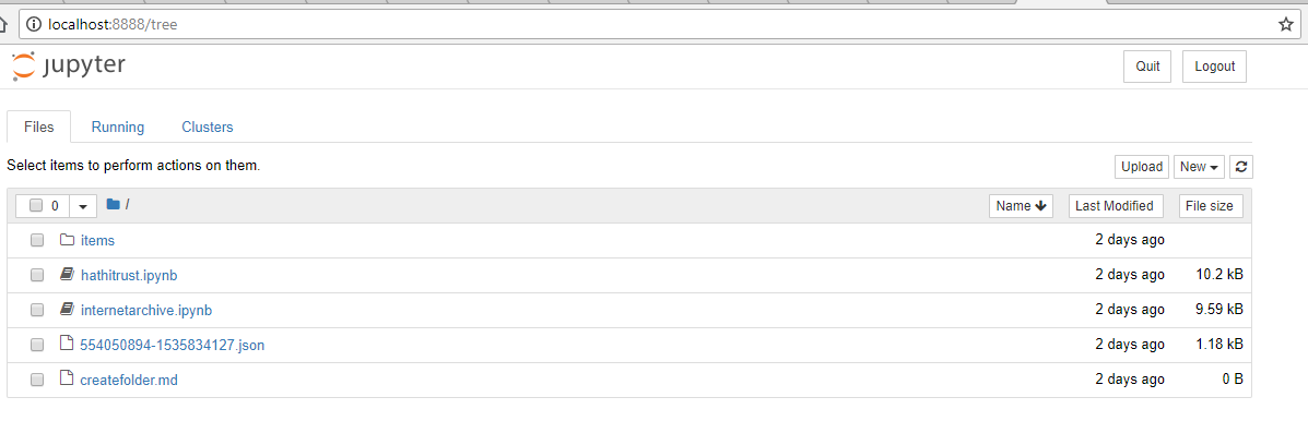
Jupyter homepage showing lesson files.
cd-ed into the unzipped lesson-files directory.
Click on the hathitrust.ipynb and internetarchive.ipynb notebooks to open them in new browser tabs. From now on, we don’t need to run any commands in the shell. The notebooks allow us to execute Python code and have full access to the computer’s file system. When you are finished, you can stop the notebook server by clicking “Quit” on the Jupyter homepage or executing ctrl+c in the shell.
HathiTrust
API Access
You need to register with HathiTrust before using the Data API. Head over to the registration portal and fill out your name, organization, and email to request access keys. You should receive an email response within a minute or so. Click the link, which will take you to a one-time page with both keys displayed.
In the hathitrust.ipynb notebook, examine the very first cell (shown below). Fill in your API tokens as directed. Then run the cell by clicking “Run” in the notebook navbar.
# Import the HT Data API wrapper
from hathitrust_api import DataAPI

# Replace placeholder strings with your HT credentials (leaving the quote marks)
ht_access_key = "YOUR_ACCESS_KEY_HERE"
ht_secret_key = "YOUR_SECRET_KEY_HERE"

# instantiate the Data API connection object
data_api = DataAPI(ht_access_key, ht_secret_key)
Create Volume List
HT allows anyone to make a collection of items—you don’t even have to be logged in! You should register for an account, however, if you want to save your list of volumes. Follow the instructions to do some full-text searches and then add selected results to a collection. Currently, HathiTrust does not have a public search API for acquiring volumes programmatically; you need to search through their web interface.
As you update a collection, HT keeps track of the associated metadata for each item in it. I have included in the lesson files the metadata for a sample lesson in JSON format. If you wanted to use the file from your own HT collection, you would navigate to your collections page and hover on the metadata link on the left to bring up the option to download as JSON as seen in the following screenshot.
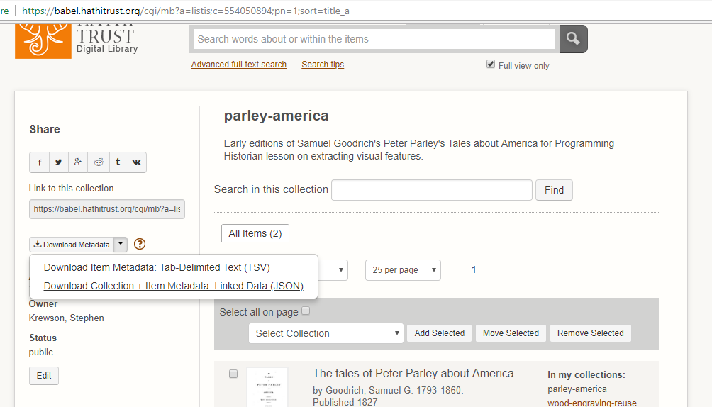
Screenshot of how to download collection metadata in JSON format.
When you have downloaded the JSON file, simply move it to the directory where you placed the Jupyter notebooks. Replace the name of the JSON file in the HT notebook with the name of your collection’s file.
The notebook shows how to use a list comprehension to get all the htitem_id strings within the gathers object that contains all the collection information.
# you can specify your collection metadata file here
metadata_path = "554050894-1535834127.json"

with open(metadata_path, "r") as fp:
    data = json.load(fp)

# a list of all unique ids in the collection
vol_ids = [item['htitem_id'] for item in data['gathers']]
Visual Feature: IMAGE_ON_PAGE
Given a list of volumes, we want to explore what visual features they have at the page level. The most recent documentation (2015) for the Data API describes a metadata object called htd:pfeat on pages 9-10. htd:pfeat is shorthand for “HathiTrust Data API: Page Features.”
htd:pfeat - the page feature key (if available):
- CHAPTER_START
- COPYRIGHT
- FIRST_CONTENT_CHAPTER_START
- FRONT_COVER
- INDEX
- REFERENCES
- TABLE_OF_CONTENTS
- TITLE
What the hathitrust-api wrapper does is make the full metadata for a HT volume available as a Python object. Given a volume’s identifier, we can request its metadata and then drill down through the page sequence into page-level information. The htd:pfeat list is associated with each page in a volume and in theory contains all features that apply to that page. In practice, there a quite a few more feature tags than the eight listed above. The one we will be working with is called IMAGE_ON_PAGE and is more abstractly visual than structural tags such as CHAPTER_START.
Tom Burton-West, a research librarian at the University of Michigan Library, works closely with HathiTrust and HTRC, HathiTrust’s Research Center. Tom told me over email that HathiTrust is provided the htd:pfeat information by Google, with whom they have worked closely since HT’s founding in 2008. A contact at Google gave Tom permission to share the following:
These tags are derived from a combination of heuristics, machine learning, and human tagging.
An example heuristic might be that the first element in the volume page sequence is almost always the FRONT_COVER. Machine learning could be used to train models to discriminate, say, between image data that is more typical of lines of prose in a Western script or of the lines in an engraving. Human tagging is the manual assignment of labels to images. The ability to view a volume’s illustrations in the EEBO and ECCO databases is an example of human tagging.
The use of “machine learning” by Google sounds somewhat mysterious. Until Google publicizes their methods, it is impossible to know all the details. However, it’s likely that the IMAGE_ON_PAGE tags were first proposed by detecting “Picture” blocks in the OCR output files (a process discussed below in the Internet Archive section). Further filtering may then be applied.
Code Walk-through
Find Pictures
We have seen how to create a list of volumes and observed that the Data API can be used to get metadata objects containing page-level experimental features. The core function in the HT notebook has the signature ht_picture_download(item_id, out_dir=None). Given a unique identifier and an optional destination directory, this function will first get the volume’s metadata from the API and convert it into JSON format. Then it loops over the page sequence and checks if the tag IMAGE_ON_PAGE is in the htd:pfeat list (if it exists).
# metadata from API in json format (different than HT collection metadata)
meta = json.loads(data_api.getmeta(item_id, json=True))

# sequence gets us each page of the scanned item in order, with any
# additional information that might be available for it
sequence = meta['htd:seqmap'][0]['htd:seq']

# list of pages with pictures (empty to start)
img_pages = []

# try/except block handles situation where no "pfeats" exist OR
# the sequence numbers are not numeric
for page in sequence:
    try:
        if 'IMAGE_ON_PAGE' in page['htd:pfeat']:
            img_pages.append(int(page['pseq']))
    except (KeyError, TypeError) as e:
        continue
Notice that we need to drill down several levels into the top-level object to get the htd:seq object, which we can iterate over.
The two exceptions I want to catch are KeyError, which occurs when the page does not have an page-level features associated with it and TypeError, which occurs when the pseq field for the page is for some reason non-numeric and thus cannot be cast to an int. If something goes wrong with a page, we just continue on to the next one. The idea is to get all the good data we can. Not to clean up inconsistencies or gaps in the item metadata.
Download Images
Once img_pages contains the complete list of pages tagged with IMAGE_ON_PAGE, we can download those pages. Note that if no out_dir is supplied to ht_picture_download(), then the function simply returns the img_pages list and does NOT download anything.
The getpageimage() API call returns a JPEG by default. We simply write out the JPEG bytes to a file in the normal way. Within the volume sub-folder (itself inside out_dir), the pages will be named 1.jpg for page 1 and so forth.
One thing to consider is our usage rate of the API. We don’t want to abuse our access by making hundreds of requests per minute. To be safe, especially if we intend to run big jobs, we wait two seconds before making each page request. This may be frustrating in the short term, but it helps avoid API throttling or banning.
for i, page in enumerate(img_pages):
    try:
		# simple status message
        print("[{}] Downloading page {} ({}/{})".format(item_id, \
			page, i+1, total_pages))

        img = data_api.getpageimage(item_id, page)

        # N.B. loop only executes if out_dir is not None
        img_out = os.path.join(out_dir, str(page) + ".jpg")

        # write out the image
        with open(img_out, 'wb') as fp:
            fp.write(img)

        # to avoid exceeding the allowed API usage
        time.sleep(2)

    except Exception as e:
        print("[{}] Error downloading page {}: {}".format(item_id, page,e))
Internet Archive
API Access
We connect to the Python API library using an Archive.org account email and password rather than API tokens. This is discussed in the Quickstart Guide. If you do not have an account, register for your “Virtual Library Card.”
In the first cell of the internetarchive.ipynb notebook, enter your credentials as directed. Run the cell to authenticate to the API.
Create Volume List
The IA Python library allows you to submit query strings and receive a list of matching key-value pairs where the word “identifier” is the key and the actual identifier is the value. The syntax for a query is explained on the Advanced Search page for IA. You can specify parameters by using a keyword like “date” or “mediatype” followed by a colon and the value you want to assign that parameter. For instance, I only want results that are texts (as opposed to video, etc.). Make sure the parameters and options you are trying to use are supported by IA’s search functionality. Otherwise you may get missing or weird results and not know why.
In the notebook, I generate a list of IA ids with the following code:
# sample search (should yield two results)
query = "peter parley date:[1825 TO 1830] mediatype:texts"
vol_ids = [result['identifier'] for result in ia.search_items(query)]
Visual Feature: Picture Blocks
Internet Archive does not release any page-level features. Instead, it makes a number of raw files from the digitization process available to users. The most important of these for our purposes is the Abbyy XML file. Abbyy is a Russian company whose FineReader software dominates the OCR market.
All recent versions of FineReader produce an XML document that associates different “blocks” with each page in the scanned document. The most common type of block is Text but there are Picture blocks as well. Here is an example block taken from an IA Abbyy XML file. The top-left (“t” and “l”) and bottom-right (“b” and “r”) corners are enough to identify the rectangular block region.
<block blockType="Picture" l="586" t="1428" r="768" b="1612">
	<region><rect l="586" t="1428" r="768" b="1612"></rect></region>
</block>
The IA equivalent to looking for IMAGE_ON_PAGE tags in HT is parsing the Abbyy XML file and iterating over each page. If there is at least one Picture block on that page, the page is flagged as possibly containing an image.
While HT’s IMAGE_ON_PAGE feature contains no information about the location of that image, the Picture blocks in the XML file are associated with a rectangular region on the page. However, since FineReader specializes in recognizing letters from Western character sets, it is much less accurate at identifying image regions. Leetaru’s project (see Overview) used the region coordinates to crop pictures, but in this lesson we will simply download the whole page.
Part of the intellectual fun of this lesson is using a noisy dataset (OCR block tags) for a largely unintended purpose: identifying pictures and not words. At some point, it will become computationally feasible to run deep learning models on every raw page image in a volume and pick out the desired type(s) of picture(s). But since most pages in most volumes are unillustrated, that is an expensive task. For now, it makes more sense to leverage the existing data we have from the OCR ingest process.
For more information on how OCR itself works and interacts with the scan process, please see Mila Oiva’s PH lesson OCR with Tesseract and ScanTailor. Errors can crop up due to skewing, artefacts, and many other problems. These errors end up affecting the reliability and precision of the “Picture” blocks. In many cases, Abbyy will estimate that blank or discolored pages are actually pictures. These incorrect block tags, while undesirable, can be dealt with using retrained convolutional neural networks. Think of the page images downloaded in this lesson as a first pass in a longer process of obtaining a clean and usable dataset of historical illustrations.
Code Walk-through
Find Pictures
Just as with HT, the core function for IA is ia_picture_download(item_id, out_dir=None).
Since it involves file I/O, the process for geting the img_pages list is more complicated than that for HT. Using the command line utility ia (which is installed with the library), you can get a sense of the available metadata files for a volume. With very few exceptions, a file with format “Abbyy GZ” should be available for volumes with media type text on Internet Archive.
These files, even when compressed, can easily be hundreds of megabytes in size! If there is an Abbyy file for the volume, we get its name and then download it. The ia.download() call uses some helpful parameters to ignore the request if the file already exists and, if not, download it without creating a nested directory. To save space, we delete the Abbyy file after parsing it.
# Use command-line client to see available metadata formats:
# `ia metadata formats VOLUME_ID`

# for this lesson, only the Abbyy file is needed
returned_files = list(ia.get_files(item_id, formats=["Abbyy GZ"]))

# make sure something got returned
if len(returned_files) > 0:
    abbyy_file = returned_files[0].name
else:
    print("[{}] Could not get Abbyy file".format(item_id))
    return None

# download the abbyy file to CWD
ia.download(item_id, formats=["Abbyy GZ"], ignore_existing=True, \
	destdir=os.getcwd(), no_directory=True)
Once we have the file, we need to parse the XML using the standard Python library. We take advantage of the fact that we can open the compressed file directly with the gzip library. Abbyy files are zero-indexed so the first page in the scan sequence has index 0. However, we have to filter out 0 since it cannot be requested from IA. IA’s exclusion of index 0 is not documented anywhere; rather, I found out through trial and error. If you see a hard-to-explain error message, try to track down the source and don’t be afraid to ask for help, whether from someone with relevant experience or at the organization itself.
# collect the pages with at least one picture block
img_pages = []

with gzip.open(abbyy_file) as fp:
    tree = ET.parse(fp)
    document = tree.getroot()
    for i, page in enumerate(document):
        for block in page:
            try:
                if block.attrib['blockType'] == 'Picture':
                    img_pages.append(i)
                    break
            except KeyError:
                continue

# 0 is not a valid page for making GET requests to IA, yet sometimes
# it's in the zipped Abbyy file
img_pages = [page for page in img_pages if page > 0]

# track for download progress report
total_pages = len(img_pages)

# OCR files are huge, so just delete once we have pagelist
os.remove(abbyy_file)
Download Images
IA’s Python wrapper does not provide a single-page download function—only bulk. This means that we will use IA’s RESTful API to get specific pages. First we construct a URL for each page that we need. Then we use the requests library to send an HTTP GET request and, if everything goes well (i.e. the code 200 is returned in the response), we write out the contents of the response to a JPEG file.
IA has been working on an alpha version of an API for image cropping and resizing that conforms to the standards of the International Image Interoperability Framework (IIIF). IIIF represents a vast improvement on the old method for single-page downloads which required downloading JP2 files, a largely unsupported archival format. Now it’s extremely simple to get a single page JPEG:
# See: https://iiif.archivelab.org/iiif/documentation
urls = ["https://iiif.archivelab.org/iiif/{}${}/full/full/0/default.jpg".format(item_id, page)
    for page in img_pages]

# no direct page download through python library, construct GET request
for i, page, url in zip(range(1,total_pages), img_pages, urls):

    rsp = requests.get(url, allow_redirects=True)

    if rsp.status_code == 200:
        print("[{}] Downloading page {} ({}/{})".format(item_id, \
			page, i+1, total_pages))

        with open(os.path.join(out_dir, str(page) + ".jpg"), "wb") as fp:
            fp.write(rsp.content)
Next Steps
Once you understand the main functions and the data unpacking code in the notebooks, feel free to run the cells in sequence or “Run All” and watch the picture pages roll in. You are encouraged to adapt these scripts and functions for your own research questions.