
Contents
- Introduction
- Imports, Uploads, and Preprocessing
- Text Enrichment with spaCy
- Analysis of Linguistic Annotations
- Conclusions
- Endnotes
Introduction
Say you have a big collection of texts. Maybe you’ve gathered speeches from the French Revolution, compiled a bunch of Amazon product reviews, or unearthed a collection of diary entries written during the first world war. In any of these cases, computational analysis can be a good way to compliment close reading of your corpus… but where should you start?
One possible way to begin is with spaCy, an industrial-strength library for Natural Language Processing (NLP) in Python. spaCy is capable of processing large corpora, generating linguistic annotations including part-of-speech tags and named entities, as well as preparing texts for further machine classification. This lesson is a ‘spaCy 101’ of sorts, a primer for researchers who are new to spaCy and want to learn how it can be used for corpus analysis. It may also be useful for those who are curious about natural language processing tools in general, and how they can help us to answer humanities research questions.
Lesson Goals
By the end of this lesson, you will be able to:
- Upload a corpus of texts to a platform for Python analysis (using Google Colaboratory)
- Use spaCy to enrich the corpus through tokenization, lemmatization, part-of-speech tagging, dependency parsing and chunking, and named entity recognition
- Conduct frequency analyses using part-of-speech tags and named entities
- Download an enriched dataset for use in future NLP analyses
Why Use spaCy for Corpus Analysis?
As the name implies, corpus analysis involves studying corpora, or large collections of documents. Typically, the documents in a corpus are representative of the group(s) a researcher is interested in studying, such as the writings of a specific author or genre. By analyzing these texts at scale, researchers can identify meaningful trends in the way language is used within the target group(s).
Though computational tools like spaCy can’t read and comprehend the meaning of texts like humans do, they excel at ‘parsing’ (analyzing sentence structure) and ‘tagging’ (labeling) them. When researchers give spaCy a corpus, it will ‘parse’ every document in the collection, identifying the grammatical categories to which each word and phrase in each text most likely belongs. NLP Algorithms like spaCy use this information to generate lexico-grammatical tags that are of interest to researchers, such as lemmas (base words), part-of-speech tags and named entities (more on these in the Part-of-Speech Analysis and Named Entity Recognition sections below). Furthermore, computational tools like spaCy can perform these parsing and tagging processes much more quickly (in a matter of seconds or minutes) and on much larger corpora (hundreds, thousands, or even millions of texts) than human readers would be able to.
Though spaCy was designed for industrial use in software development, researchers also find it valuable for several reasons:
- It’s easy to set up and use spaCy’s Trained Models and Pipelines; there is no need to call a wide range of packages and functions for each individual task
- It uses fast and accurate algorithms for text-processing tasks, which are kept up-to-date by the developers so it’s efficient to run
- It performs better on text-splitting tasks than Natural Language Toolkit (NLTK), because it constructs syntactic trees for each sentence
You may still be wondering: What is the value of extracting language data such as lemmas, part-of-speech tags, and named entities from a corpus? How can this data help researchers answer meaningful humanities research questions? To illustrate, let’s look at the example corpus and questions developed for this lesson.
Dataset: Michigan Corpus of Upper-Level Student Papers
The Michigan Corpus of Upper-Level Student Papers (MICUSP) is a corpus of 829 high-scoring academic writing samples from students at the University of Michigan. The texts come from 16 disciplines and seven genres, all were written by senior undergraduate or graduate students and received an A-range score in a university course.1 The texts and their metadata are publicly available on MICUSP Simple, an online interface which allows users to search for texts by a range of fields (for example genre, discipline, student level, textual features) and conduct simple keyword analyses across disciplines and genres.
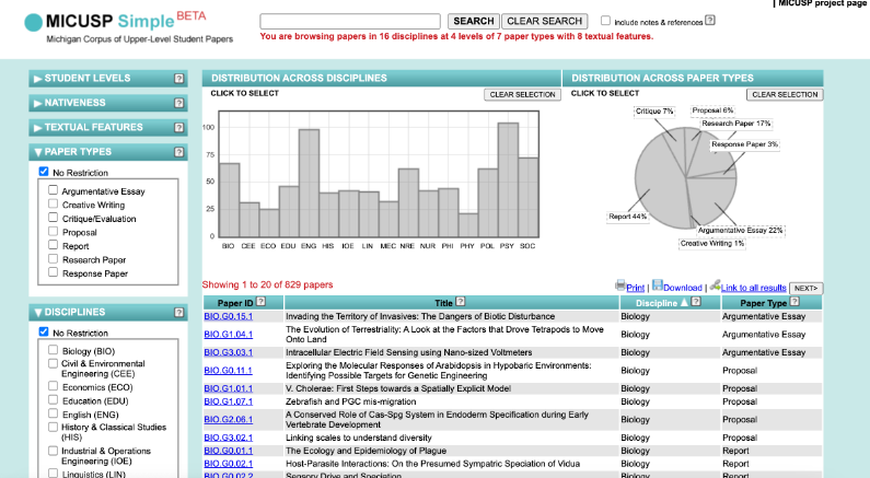
Figure 1: MICUSP Simple Interface
Metadata from the corpus is available to download in .csv format. The text files can be retrieved through webscraping, a process explained further in Jeri Wieringa’s Intro to BeautifulSoup lesson, a Programming Historian lesson which remains methodologically useful even if it has been retired due to changes to the scraped website.
Given its size and robust metadata, MICUSP has become a valuable tool for researchers seeking to study student writing computationally. Notably, Jack Hardy and Ute Römer2 use MICUSP to study language features that indicate how student writing differs across disciplines. Laura Aull compares usages of stance markers across student genres3, and Sugene Kim highlights discrepancies between prescriptive grammar rules and actual language use in student work4. Like much corpus analysis research, these studies are predicated on the fact that computational analysis of language patterns — the discrete lexico-grammatical practices students employ in their writing — can yield insights into larger questions about academic writing. Given its value in discovering linguistic annotations, spaCy is well-poised to conduct this type of analysis on MICUSP data.
This lesson will explore a subset of documents from MICUSP: 67 Biology papers and 98 English papers. Writing samples in this select corpus belong to all seven MICUSP genres: Argumentative Essay, Creative Writing, Critique/Evaluation, Proposal, Report, Research Paper, and Response Paper. This select corpus .txt_files.zip and the associated metadata.csv are available to download as sample materials for this lesson. The dataset has been culled from the larger corpus in order to investigate the differences between two distinct disciplines of academic writing (Biology and English). It is also a manageable size for the purposes of this lesson.
Quick note on corpus size and processing speed: spaCy is able to process jobs of up to 1 million characters, so it can be used to process the full MICUSP corpus, or other corpora containing hundreds or thousands of texts. You are more than welcome to retrieve the entire MICUSP corpus with this webscraping code and using that dataset for the analysis.
Research Questions: Linguistic Differences Within Student Paper Genres and Disciplines
This lesson will describe how spaCy’s utilities in stopword removal, tokenization, and lemmatization can assist in (and hinder) the preparation of student texts for analysis. You will learn how spaCy’s ability to extract linguistic annotations such as part-of-speech tags and named entities can be used to compare conventions within subsets of a discursive community of interest. The lesson focuses on lexico-grammatical features that may indicate genre and disciplinary differences in academic writing.
The following research questions will be investigated:
1: Do students use certain parts-of-speech more frequently in Biology texts versus English texts, and does this linguistic discrepancy signify differences in disciplinary conventions?
Prior research has shown that even when writing in the same genres, writers in the sciences follow different conventions than those in the humanities. Notably, academic writing in the sciences has been characterized as informational, descriptive, and procedural, while scholarly writing in the humanities is narrativized, evaluative, and situation-dependent (that is, focused on discussing a particular text or prompt)5. By deploying spaCy on the MICUSP texts, researchers can determine whether there are any significant differences between the part-of-speech tag frequencies in English and Biology texts. For example, we might expect students writing Biology texts to use more adjectives than those in the humanities, given their focus on description. Conversely, we might suspect English texts to contain more verbs and verb auxiliaries, indicating a more narrative structure. To test these hypotheses, you’ll learn to analyze part-of-speech counts generated by spaCy, as well as to explore other part-of-speech count differences that could prompt further investigation.
2: Do students use certain named entities more frequently in different academic genres, and do these varying word frequencies signify broader differences in genre conventions?
As with disciplinary differences, research has shown that different genres of writing have their own conventions and expectations. For example, explanatory genres such as research papers, proposals and reports tend to focus on description and explanation, whereas argumentative and critique-driven texts are driven by evaluations and arguments6. By deploying spaCy on the MICUSP texts, researchers can determine whether there are any significant differences between the named entity frequencies in texts within the seven different genres represented (Argumentative Essay, Creative Writing, Critique/Evaluation, Proposal, Report, Research Paper, and Response Paper). We may suspect that argumentative genres engage more with people or works of art, since these could be entities serving to support their arguments or as the subject of their critiques. Conversely, perhaps dates and numbers are more prevalent in evidence-heavy genres, such as research papers and proposals. To test these hypotheses, you’ll learn to analyze the nouns and noun phrases spaCy has tagged as ‘named entities.’
In addition to exploring the research questions above, this lesson will address how a dataset enriched by spaCy can be exported in a usable format for further machine learning tasks including sentiment analysis or topic modeling.
Prerequisites
You should have some familiarity with Python or a similar coding language. For a brief introduction or refresher, work through some of the Programming Historian’s introductory Python tutorials. You should also have basic knowledge of spreadsheet (.csv) files, as this lesson will primarily use data in a similar format called a pandas DataFrame. Halle Burns’s lesson Crowdsourced-Data Normalization with Python and Pandas provides an overview of creating and manipulating datasets using pandas.
The code for this lesson has been prepared as a Jupyter Notebook that is customized and ready to run in Google Colaboratory.
Jupyter Notebooks are browser-based, interactive computing environments for Python. Colaboratory is a Google platform which allows you to run cloud-hosted Jupyter Notebooks, with additional built-in features. If you’re new to coding and aren’t working with sensitive data, Google Colab may be the best option for you. There is a brief Colab tutorial from Google available for beginners.
You can also download the lesson code and run it on your local machine. The practical steps for running the code locally are the same except when it comes to installing packages and retrieving and downloading files. These divergences are marked in the notebook. Quinn Dombrowski, Tassie Gniady, and David Kloster’s lesson Introduction to Jupyter Notebooks covers the necessary background for setting up and using a Jupyter Notebook with Anaconda.
It is also recommended, though not required, that before starting this lesson you learn about common text mining methods. Heather Froehlich’s lesson Corpus Analysis with AntConc shares tips for working with plain text files and outlines possibilities for exploring keywords and collocations in a corpora. William J. Turkel and Adam Crymble’s lesson Counting Word Frequencies with Python describes the process of counting word frequencies, a practice this lesson will adapt to count part-of-speech and named entity tags.
No prior knowledge of spaCy is required. For a quick overview, go to the spaCy 101 page from the library’s developers.
Imports, Uploads, and Preprocessing
Import Packages
Import spaCy and related packages into your Colab environment.
# Install and import spaCy
import spacy

# Load spaCy visualizer
from spacy import displacy

# Import os to upload documents and metadata
import os

# Import pandas DataFrame packages
import pandas as pd

# Import graphing package
import plotly.graph_objects as go
import plotly.express as px

# Import drive and files to facilitate file uploads
from google.colab import files
Upload Text Files
After all necessary packages have been imported, it is time to upload the data for analysis with spaCy. Prior to running the code below, make sure the MICUSP text files you are going to analyze are saved to your local machine.
Run the code below to select multiple files to upload from a local folder:
uploaded_files = files.upload()
When the cell has run, navigate to where you stored the MICUSP text files. Select all the files of interest and click Open. The text files should now be uploaded to your Google Colab session.
Now we have files upon which we can perform analysis. To check what form of data we are working with, you can use the type() function.
type(uploaded_files)
It should return that your files are contained in a dictionary, where keys are the filenames and values are the content of each file.
Next, we’ll make the data easier to manage by inserting it into a pandas DataFrame. As the files are currently stored in a dictionary, use the DataFrame.from_dict() function to append them to a new DataFrame:
paper_df = pd.DataFrame.from_dict(uploaded_files, orient='index')
paper_df.head()
Use the .head() function to call the first five rows of the DataFrame and check that the filenames and text are present. You will also notice some strange characters at the start of each row of text; these are byte string characters (b' or b") related to the encoding, and they will be removed below.
This table shows the initial DataFrame with filenames and texts. These are the first five rows of the student text DataFrame, including columns for the title of each text and the body of each text, without column header names and with byte string characters at start of each line.
| 0 | |
|---|---|
| BIO.G0.01.1.txt | b”Introduction\xe2\x80\xa6\xe2\x80\xa6\xe2\x80… |
| BIO.G0.02.1.txt | b’ Ernst Mayr once wrote, sympatric speci… |
| BIO.G0.02.2.txt | b” Do ecological constraints favour certa… |
| BIO.G0.02.3.txt | b” Perhaps one of the most intriguing va… |
| BIO.G0.02.4.txt | b” The causal link between chromosomal re… |
From here, you can reset the index (the very first column of the DataFrame) so it is a true index, rather than the list of filenames. The filenames will become the first column and the texts become the second, making data wrangling easier later.
# Reset index and add column names to make wrangling easier
paper_df = paper_df.reset_index()
paper_df.columns = ["Filename", "Text"]
Check the head of the DataFrame again to confirm this process has worked.
Pre-process Text Files
If you’ve done any computational analysis before, you’re likely familiar with the term ‘cleaning’, which covers a range of procedures such as lowercasing, punctuation removal, and stopword removal. Such procedures are used to standardize data and make it easier for computational tools to interpret it. In the next step, you will convert the uploaded files from byte strings into Unicode strings so that spaCy can process them and replace extra spaces with single spaces.
First, you will notice that each text in your DataFrame starts with b' or b". This indicates that the data has been read as ‘byte strings’, or strings which represent as sequence of bytes. 'b"Hello", for example, corresponds to the sequence of bytes 104, 101, 108, 108, 111. To analyze the texts with spaCy, we need them to be Unicode strings, where the characters are individual letters.
Converting from bytes to strings is a quick task using str.decode(). Within the parentheses, we specify the encoding parameter, UTF-8 (Unicode Transformation Format - 8 bits) which guides the transformation from bytes to Unicode strings. For a more thorough breakdown of encoding in Python, check out this lesson.
paper_df['Text'] = paper_df['Text'].str.decode('utf-8')
paper_df.head()
Here, we generate a decoded DataFrame with filenames and texts. This table shows the first five rows of student texts DataFrame, including columns for the Filename and the Text of each paper, with byte string characters removed.
| Filename | Text | |
|---|---|---|
| 0 | BIO.G0.01.1.txt | Introduction……………………………………………………..1 Brief Hist… |
| 1 | BIO.G0.02.1.txt | Ernst Mayr once wrote, sympatric speciation is… |
| 2 | BIO.G0.02.2.txt | Do ecological constraints favour certain perce… |
| 3 | BIO.G0.02.3.txt | Perhaps one of the most intriguing varieties o… |
| 4 | BIO.G0.02.4.txt | The causal link between chromosomal rearrangem… |
Additionally, the beginnings of some of the texts may also contain extra spaces (indicated by \t or \n). These characters can be replaced by a single space using the str.replace() method.
paper_df['Text'] = paper_df['Text'].str.replace('\s+', ' ', regex=True).str.strip()
Further cleaning is not necessary before running running spaCy, and some common cleaning processes will, in fact, skew your results. For example, punctuation markers help spaCy parse grammatical structures and generate part-of-speech tags and dependency trees. Recent scholarship suggests that removing stopwords only superficially improves tasks like topic modeling, that retaining stopwords can support clustering and classification7. At a later stage of this lesson, you will learn to remove stopwords so you can compare its impact on spaCy results.
Upload and Merge Metadata Files
Next you will retrieve the metadata about the MICUSP corpus: the discipline and genre information connected to the student texts. Later in this lesson, you will use spaCy to trace differences across genre and disciplinary categories.
In your Colab, run the following code to upload the .csv file from your local machine.
metadata = files.upload()
Then convert the uploaded .csv file to a second DataFrame, dropping any empty columns.
metadata_df = pd.read_csv('metadata.csv')
metadata_df = metadata_df.dropna(axis=1, how='all')
The metadata DataFrame will include columns headed paper metadata-ID, title, discpline and type. This table displays the first five rows:
| PAPER ID | TITLE | DISCIPLINE | PAPER TYPE | |
|---|---|---|---|---|
| 0 | BIO.G0.15.1 | Invading the Territory of Invasives: The Dange… | Biology | Argumentative Essay |
| 1 | BIO.G1.04.1 | The Evolution of Terrestriality: A Look at the… | Biology | Argumentative Essay |
| 2 | BIO.G3.03.1 | Intracellular Electric Field Sensing using Nan… | Biology | Argumentative Essay |
| 3 | BIO.G0.11.1 | Exploring the Molecular Responses of Arabidops… | Biology | Proposal |
| 4 | BIO.G1.01.1 | V. Cholerae: First Steps towards a Spatially E… | Biology | Proposal |
Notice that the paper IDs in this DataFrame are almost the same as the paper filenames in the corpus DataFrame. We’re going to make them match exactly so we can merge the two DataFrames together on this column; in effect, linking each text with their title, discipline and genre.
To match the columns, we’ll remove the .txt extension from the end of each filename in the corpus DataFrame using a simple str.replace function. This function searches for every instance of the phrase .txt in the Filename column and replaces it with nothing (in effect, removing it). In the metadata DataFrame, we’ll rename the paper ID column Filename.
# Remove .txt from title of each paper
paper_df['Filename'] = paper_df['Filename'].str.replace('.txt', '')

# Rename column from paper ID to Title
metadata_df.rename(columns={"PAPER ID": "Filename"}, inplace=True)
Now it is possible to merge the papers and metadata into a single DataFrame:
final_paper_df = metadata_df.merge(paper_df,on='Filename')
Check the first five rows to make sure each has a filename, title, discipline, paper type and text (the full paper). At this point, you’ll also see that any extra spaces have been removed from the beginning of the texts.
| Filename | TITLE | DISCIPLINE | PAPER TYPE | Text | |
|---|---|---|---|---|---|
| 0 | BIO.G0.15.1 | Invading the Territory of Invasives: The Dange… | Biology | Argumentative Essay | New York City, 1908: different colors of skin … |
| 1 | BIO.G1.04.1 | The Evolution of Terrestriality: A Look at the… | Biology | Argumentative Essay | The fish-tetrapod transition has been called t… |
| 2 | BIO.G3.03.1 | Intracellular Electric Field Sensing using Nan… | Biology | Argumentative Essay | Intracellular electric fields are of great int… |
| 3 | BIO.G0.11.1 | Exploring the Molecular Responses of Arabidops… | Biology | Proposal | Environmental stresses to plants have been stu… |
| 4 | BIO.G1.01.1 | V. Cholerae: First Steps towards a Spatially E… | Biology | Proposal | The recurrent cholera pandemics have been rela… |
The resulting DataFrame is now ready for analysis.
Text Enrichment with spaCy
Creating Doc Objects
To use spaCy, the first step is to load one of spaCy’s Trained Models and Pipelines which will be used to perform tokenization, part-of-speech tagging, and other text enrichment tasks. A wide range of options are available (see the full list here), and they vary based on size and language.
We’ll use en_core_web_sm, which has been trained on written web texts. It may not perform as accurately as the those trained on medium and large English language models, but it will deliver results most efficiently. Once we’ve loaded en_core_web_sm, we can check what actions it performs; parser, tagger, lemmatizer, and ner, should be among those listed.
nlp = spacy.load('en_core_web_sm')

print(nlp.pipe_names)
Now that the nlp function is loaded, let’s test out its capacities on a single sentence. Calling the nlp function on a single sentence yields a Doc object. This object stores not only the original text, but also all of the linguistic annotations obtained when spaCy processed the text.
sentence = "This is 'an' example? sentence"

doc = nlp(sentence)
Next we can call on the Doc object to get the information we’re interested in. The command below loops through each token in a Doc object and prints each word in the text along with its corresponding part-of-speech:
for token in doc:
    print(token.text, token.pos_)
This PRON
is AUX
' PUNCT
an DET
' PUNCT
example NOUN
? PUNCT
sentence NOUN
Let’s try the same process on the student texts. As we’ll be calling the NLP function on every text in the DataFrame, we should first define a function that runs nlp on whatever input text is given. Functions are a useful way to store operations that will be run multiple times, reducing duplications and improving code readability.
def process_text(text):
    return nlp(text)
After the function is defined, use .apply() to apply it to every cell in a given DataFrame column. In this case, nlp will run on each cell in the Text column of the final_paper_df DataFrame, creating a Doc object from every student text. These Doc objects will be stored in a new column of the DataFrame called Doc.
Running this function takes several minutes because spaCy is performing all the parsing and tagging tasks on each text. However, when it is complete, we can simply call on the resulting Doc objects to get parts-of-speech, named entities, and other information of interest, just as in the example of the sentence above.
final_paper_df['Doc'] = final_paper_df['Text'].apply(process_text)
Text Reduction
Tokenization
A critical first step spaCy performs is tokenization, or the segmentation of strings into individual words and punctuation markers. Tokenization enables spaCy to parse the grammatical structures of a text and identify characteristics of each word-like part-of-speech.
To retrieve a tokenized version of each text in the DataFrame, we’ll write a function that iterates through any given Doc object and returns all functions found within it. This can be accomplished by simply putting a define wrapper around a for loop, similar to the one written above to retrieve the tokens and parts-of-speech from a single sentence.
def get_token(doc):
    for token in doc:
        return token.text
However, there’s a way to write the same function that makes the code more readable and efficient. This is called List Comprehension, and it involves condensing the for loop into a single line of code and returning a list of tokens within each text it processes:
def get_token(doc):
    return [(token.text) for token in doc]
As with the function used to create Doc objects, the token function can be applied to the DataFrame. In this case, we will call the function on the Doc column, since this is the column which stores the results from the processing done by spaCy.
final_paper_df['Tokens'] = final_paper_df['Doc'].apply(get_token)
If we compare the Text and Tokens column, we find a couple of differences. In the table below, you’ll notice that most importantly, the words, spaces, and punctuation markers in the Tokens column are separated by commas, indicating that each have been parsed as individual tokens. The text in the Tokens column is also bracketed; this indicates that tokens have been generated as a list.
| Text | Tokens | |
|---|---|---|
| 0 | New York City, 1908: different colors of skin … | [New, York, City, ,, 1908, :, different, color… |
| 1 | The fish-tetrapod transition has been called t… | [The, fish, -, tetrapod, transition, has, been… |
| 2 | Intracellular electric fields are of great int… | [Intracellular, electric, fields, are, of, gre… |
| 3 | Environmental stresses to plants have been stu… | [Environmental, stresses, to, plants, have, be… |
| 4 | The recurrent cholera pandemics have been rela… | [The, recurrent, cholera, pandemics, have, bee… |
Lemmatization
Another process performed by spaCy is lemmatization, or the retrieval of the dictionary root word of each word (for example “brighten” for “brightening”). We’ll perform a similar set of steps to those above to create a function to call the lemmas from the Doc object, then apply it to the DataFrame.
def get_lemma(doc):
    return [(token.lemma_) for token in doc]

final_paper_df['Lemmas'] = final_paper_df['Doc'].apply(get_lemma)
Lemmatization can help reduce noise and refine results for researchers who are conducting keyword searches. For example, let’s compare counts of the word “write” in the original Tokens column and in the lemmatized Lemmas column.
print(f'"Write" appears in the text tokens column ' + str(final_paper_df['Tokens'].apply(lambda x: x.count('write')).sum()) + ' times.')
print(f'"Write" appears in the lemmas column ' + str(final_paper_df['Lemmas'].apply(lambda x: x.count('write')).sum()) + ' times.')
In reponse to this command, spaCy prints the following counts:
"Write" appears in the text tokens column 40 times.
"Write" appears in the lemmas column 310 times.
As expected, there are more instances of “write” in the Lemmas column, as the lemmatization process has grouped inflected word forms (writing, writer) into the base word “write.”
Text Annotation
Part-of-Speech Tagging
spaCy facilitates two levels of part-of-speech tagging: coarse-grained tagging, which predicts the simple universal part-of-speech of each token in a text (such as noun, verb, adjective, adverb), and detailed tagging, which uses a larger, more fine-grained set of part-of-speech tags (for example 3rd person singular present verb). The part-of-speech tags used are determined by the English language model we use. In this case, we’re using the small English model, and you can explore the differences between the models on spaCy’s website.
We can call the part-of-speech tags in the same way as the lemmas. Create a function to extract them from any given Doc object and apply the function to each Doc object in the DataFrame. The function we’ll create will extract both the coarse- and fine-grained part-of-speech for each token (token.pos_ and token.tag_, respectively).
def get_pos(doc):
    return [(token.pos_, token.tag_) for token in doc]

final_paper_df['POS'] = final_paper_df['Doc'].apply(get_pos)
We can create a list of the part-of-speech columns to review them further. The first (coarse-grained) tag corresponds to a generally recognizable part-of-speech such as a noun, adjective, or punctuation mark, while the second (fine-grained) category are a bit more difficult to decipher.
list(final_paper_df['POS'])
Here’s an excerpt from spaCy’s list of coarse- and fine-grained part-of-speech tags that appear in the student texts, including PROPN, NNP and NUM, CD among other pairs:
[[('PROPN', 'NNP'),
 ('PROPN', 'NNP'),
 ('PROPN', 'NNP'),
 ('PUNCT', ','),
 ('NUM', 'CD'),
 ('PUNCT', ':'),
 ('ADJ', 'JJ'),
 ('NOUN', 'NNS'),
 ('ADP', 'IN'),
 ('NOUN', 'NN'),
 ('NOUN', 'NN'),
 ('ADP', 'IN'),
 ('DET', 'DT'),
 ...]]
Fortunately, spaCy has a built-in function called explain that can provide a short description of any tag of interest. If we try it on the tag IN using spacy.explain("IN"), the output reads conjunction, subordinating or preposition.
In some cases, you may want to get only a set of part-of-speech tags for further analysis, like all of the proper nouns. A function can be written to perform this task, extracting only words which have been fitted with the proper noun tag.
def extract_proper_nouns(doc):
    return [token.text for token in doc if token.pos_ == 'PROPN']

final_paper_df['Proper_Nouns'] = final_paper_df['Doc'].apply(extract_proper_nouns)
Listing the nouns in each text can help us ascertain the texts’ subjects. Let’s list the nouns in two different texts, the text located in row 3 of the DataFrame and the text located in row 163.
list(final_paper_df.loc[[3, 163], 'Proper_Nouns'])
The first text in the list includes botany and astronomy concepts; this is likely to have been written for a biology course.
[['Mars',
 'Arabidopsis',
 'Arabidopsis',
 'LEA',
 'COR',
 'LEA',
 'NASA',
 ...]]
In contrast, the second text appears to be an analysis of Shakespeare plays and movie adaptations, likely written for an English course.
[['Shakespeare',
 'Bard',
 'Julie',
 'Taymor',
 'Titus',
 'Shakespeare',
 'Titus',
 ...]]
Along with assisting content analyses, extracting nouns have been shown to help build more efficient topic models8.
Dependency Parsing
Closely related to part-of-speech tagging is ‘dependency parsing’, wherein spaCy identifies how different segments of a text are related to each other. Once the grammatical structure of each sentence is identified, visualizations can be created to show the connections between different words. Since we are working with large texts, our code will break down each text into sentences (spans) and then create dependency visualizers for each span. We can then visualize the span of once sentence at a time.
doc = final_paper_df['Doc'][5]
sentences = list(doc.sents)
sentence = sentences[1]
displacy.render(sentence, style="dep", jupyter=True)
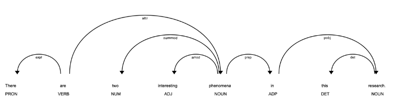
Figure 2: Dependency parsing example from one sentence of one text in corpus
If you’d like to review the output of this code as raw .html, you can download it here and open it with your browser. Here, spaCy has identified relationships between pronouns, verbs, nouns and other parts of speech in one sentence. For example, both “two” and “interesting” modify the noun “phenomena,” and the pronoun “There” is an expletive filling the noun position before “are” without adding meaning to the sentence.
Dependency parsing makes it easy to see how removing stopwords can impact spaCy’s depiction of the grammatical structure of texts. Let’s compare to a dependency parsing where stopwords are removed. To do so, we’ll create a function to remove stopwords from the Doc object, create a new Doc object without stopwords, and extract the part-of-speech tokens from the same sentence in the same text. Then we’ll create a visualization for the dependency parsing for the same sentence as above, this time without stopwords.
def extract_stopwords(doc):
    return [token.text for token in doc if token.text not in nlp.Defaults.stop_words]

final_paper_df['Tokens_NoStops'] = final_paper_df['Doc'].apply(extract_stopwords)

final_paper_df['Text_NoStops'] = [' '.join(map(str, l)) for l in final_paper_df['Tokens_NoStops']]

final_paper_df['Doc_NoStops'] = final_paper_df['Text_NoStops'].apply(process_text)

doc = final_paper_df['Doc_NoStops'][5]
sentences = list(doc.sents)
sentence = sentences[0]

displacy.render(sentence, style='dep', jupyter=True)
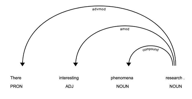
Figure 3: Dependency parsing example from one sentence of one text in corpus without stopwords
If you’d like to review the output of this code as raw .html, you can download it here. In this example, the verb of the sentence “are” has been removed, along with the adjective “two” and the words “in this” that made up the prepositional phrases. Not only do these removals prevent the sentence from being legible, but they also render some of the dependencies inaccurate; “phenomena research” is here identified as a compound noun, and “interesting” as modifying research instead of phenomena.
This example demonstrates what can be lost in analysis when stopwords are removed, especially when investigating the relationships between words in a text or corpus. Since part-of-speech tagging and named entity recognition are predicated on understanding relationships between words, it’s best to keep stopwords so spaCy can use all available linguistic units during the tagging process.
Dependency parsing also enables the extraction of larger chunks of text, like noun phrases. Let’s try it out:
def extract_noun_phrases(doc):
    return [chunk.text for chunk in doc.noun_chunks]

final_paper_df['Noun_Phrases'] = final_paper_df['Doc'].apply(extract_noun_phrases)
Calling the first row in the Noun_Phrases column will reveal the words spaCy has classified as noun phrases. In this example, spaCy has identified a wide range of nouns and nouns with modifiers, from locations (“New York City”) to phrases with adjectival descriptors (“the great melting pot”):
['New York City',
'different colors',
'skin swirl',
'the great melting pot',
'a cultural medley',
'such a metropolis',
'every last crevice',
'Earth',
'time',
'people',
'an unprecedented uniformity',
'discrete identities',
'Our heritages',
'the history texts',
  ...]]
Named Entity Recognition
Finally, spaCy can tag named entities in the text, such as names, dates, organizations, and locations. Call the full list of named entities and their descriptions using this code:
labels = nlp.get_pipe("ner").labels

for label in labels:
    print(label + ' : ' + spacy.explain(label))
spaCy lists the named entity tags that it recognizes, alongside their descriptions:
CARDINAL : Numerals that do not fall under another type
DATE : Absolute or relative dates or periods
EVENT : Named hurricanes, battles, wars, sports events, etc.
FAC : Buildings, airports, highways, bridges, etc.
GPE : Countries, cities, states
LANGUAGE : Any named language
LAW : Named documents made into laws.
LOC : Non-GPE locations, mountain ranges, bodies of water
MONEY : Monetary values, including unit
NORP : Nationalities or religious or political groups
ORDINAL : "first", "second", etc.
ORG : Companies, agencies, institutions, etc.
PERCENT : Percentage, including "%"
PERSON : People, including fictional
PRODUCT : Objects, vehicles, foods, etc. (not services)
QUANTITY : Measurements, as of weight or distance
TIME : Times smaller than a day
WORK_OF_ART : Titles of books, songs, etc.
We’ll create a function to extract the named entity tags from each Doc object and apply it to the Doc objects in the DataFrame, storing the named entities in a new column:
def extract_named_entities(doc):
    return [ent.label_ for ent in doc.ents]

final_paper_df['Named_Entities'] = final_paper_df['Doc'].apply(extract_named_entities)
final_paper_df['Named_Entities']
We can add another column with the words and phrases identified as named entities:
def extract_named_entities(doc):
    return [ent for ent in doc.ents]

final_paper_df['NE_Words'] = final_paper_df['Doc'].apply(extract_named_entities)
final_paper_df['NE_Words']
Let’s visualize the words and their named entity tags in a single text. Call the first text’s Doc object and use displacy.render to visualize the text with the named entities highlighted and tagged:
doc = final_paper_df['Doc'][1]
displacy.render(doc, style='ent', jupyter=True)
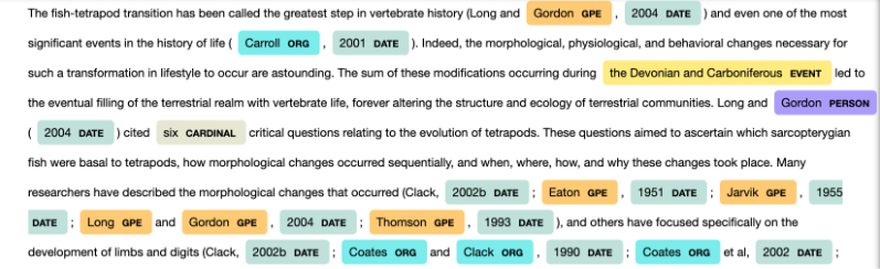
Figure 4: Visualization of one text with named entity tags
If you’d like to review the output of this code as raw .html, you can download it here. Named entity recognition enables researchers to take a closer look at the ‘real-world objects’ that are present in their texts. The rendering allows for close-reading of these entities in context, their distinctions helpfully color-coded. In addition to studying named entities that spaCy automatically recognizes, you can use a training dataset to update the categories or create a new entity category, as in this example.
Download Enriched Dataset
To save the dataset of doc objects, text reductions and linguistic annotations generated with spaCy, download the final_paper_df DataFrame to your local computer as a .csv file:
# Save DataFrame as csv (in Google Drive)
final_paper_df.to_csv('MICUSP_papers_with_spaCy_tags.csv')

# Download csv to your computer from Google Drive
files.download('MICUSP_papers_with_spaCy_tags.csv')
Analysis of Linguistic Annotations
Why are spaCy’s linguistic annotations useful to researchers? Below are two examples of how researchers can use data about the MICUSP corpus, produced through spaCy, to draw conclusions about discipline and genre conventions in student academic writing. We will use the enriched dataset generated with spaCy for these examples.
Part-of-Speech Analysis
In this section, we’ll analyze the part-of-speech tags extracted by spaCy to answer the first research question: Do students use certain parts-of-speech more frequently in Biology texts versus English texts, and does this signify differences in disciplinary conventions?
spaCy counts the number of each part-of-speech tag that appears in each document (for example the number of times the NOUN tag appears in a document). This is called using doc.count_by(spacy.attrs.POS). Here’s how it works on a single sentence:
# Create Doc object from single sentence
doc = nlp("This is 'an' example? sentence")

# Print counts of each part of speech in sentence
print(doc.count_by(spacy.attrs.POS))
Upon these commands, spaCy creates a Doc object from our sentence, then prints counts of each part-of-speech along with corresponding part-of-speech indices, for example:
{95: 1, 87: 1, 97: 3, 90: 1, 92: 2}
spaCy generates a dictionary where the values represent the counts of each part-of-speech term found in the text. The keys in the dictionary correspond to numerical indices associated with each part-of-speech tag. To make the dictionary more legible, let’s associate the numerical index values with their corresponding part of speech tags. In the example below, it’s now possible to see which parts-of-speech tags correspond to which counts:
{'AUX': 1, 'DET': 1, 'NOUN': 2, 'PRON': 1, 'PUNCT': 3}
To get the same type of dictionary for each text in a DataFrame, a function can be created to nest the above for loop. First, we’ll create a new DataFrame for the purposes of part-of speech analysis, containing the text filenames, disciplines, and Doc objects. We can then apply the function to each Doc object in the new DataFrame. In this case (and above), we are interested in the simpler, coarse-grained parts of speech.
num_list = []

# Create new DataFrame for analysis purposes
pos_analysis_df = final_paper_df[['Filename','DISCIPLINE', 'Doc']]

def get_pos_tags(doc):
    dictionary = {}
    num_pos = doc.count_by(spacy.attrs.POS)
    for k,v in sorted(num_pos.items()):
        dictionary[doc.vocab[k].text] = v
    num_list.append(dictionary)

pos_analysis_df['C_POS'] = pos_analysis_df['Doc'].apply(get_pos_tags)
From here, we’ll take the part-of-speech counts and put them into a new DataFrame where we can calculate the frequency of each part-of-speech per document. In the new DataFrame, if a paper does not contain a particular part-of-speech, the cell will read NaN (Not a Number).
pos_counts = pd.DataFrame(num_list)
columns = list(pos_counts.columns)
idx = 0
new_col = pos_analysis_df['DISCIPLINE']
pos_counts.insert(loc=idx, column='DISCIPLINE', value=new_col)
pos_counts.head()
This table shows the DataFrame including appearance counts of each part-of-speech in English and Biology papers. Notice that our column headings define the paper discipline and the part-of-speech tags counted.
| DISCIPLINE | ADJ | ADP | ADV | AUX | CCONJ | DET | INTJ | NOUN | NUM | PART | PRON | PROPN | PUNCT | SCONJ | VERB | SYM | X | |
|---|---|---|---|---|---|---|---|---|---|---|---|---|---|---|---|---|---|---|
| 0 | Biology | 180 | 174 | 62 | 106 | 42 | 137 | 1 | 342 | 29 | 29 | 41 | 101 | 196 | 16 | 139 | NaN | NaN |
| 1 | Biology | 421 | 458 | 174 | 253 | 187 | 389 | 1 | 868 | 193 | 78 | 121 | 379 | 786 | 99 | 389 | 1.0 | 2.0 |
| 2 | Biology | 163 | 171 | 63 | 91 | 51 | 148 | 1 | 362 | 6 | 31 | 23 | 44 | 134 | 15 | 114 | 4.0 | 1.0 |
| 3 | Biology | 318 | 402 | 120 | 267 | 121 | 317 | 1 | 908 | 101 | 93 | 128 | 151 | 487 | 92 | 387 | 4.0 | NaN |
| 4 | Biology | 294 | 388 | 97 | 142 | 97 | 299 | 1 | 734 | 89 | 41 | 36 | 246 | 465 | 36 | 233 | 1.0 | 7.0 |
| … | … | … | … | … | … | … | … | … | … | … | … | … | … | … | … | … | … | … |
| 160 | English | 943 | 1164 | 365 | 512 | 395 | 954 | 3 | 2287 | 98 | 315 | 530 | 406 | 1275 | 221 | 1122 | 15.0 | 8.0 |
| 161 | English | 672 | 833 | 219 | 175 | 202 | 650 | 1 | 1242 | 30 | 168 | 291 | 504 | 595 | 75 | 570 | NaN | 3.0 |
| 162 | English | 487 | 715 | 175 | 240 | 324 | 500 | 2 | 1474 | 55 | 157 | 334 | 226 | 820 | 147 | 691 | 7.0 | 5.0 |
| 163 | English | 68 | 94 | 23 | 34 | 26 | 79 | 3 | 144 | 2 | 25 | 36 | 54 | 80 | 22 | 69 | 1.0 | 2.0 |
| 164 | English | 53 | 86 | 27 | 28 | 19 | 90 | 1 | 148 | 6 | 15 | 37 | 43 | 80 | 15 | 67 | NaN | NaN |
Now you can calculate the amount of times, on average, that each part-of-speech appears in Biology versus English papers. To do so, you use the .groupby() and .mean() functions to group all part-of-speech counts from the Biology texts together and calculate the mean usage of each part-of-speech, before doing the same for the English texts. The following code also rounds the counts to the nearest whole number:
average_pos_df = pos_counts.groupby(['DISCIPLINE']).mean()

average_pos_df = average_pos_df.round(0)

average_pos_df = average_pos_df.reset_index()

average_pos_df
Our DataFrame now contains average counts of each part-of-speech tag within each discipline (Biology and English):
| DISCIPLINE | ADJ | ADP | ADV | AUX | CCONJ | DET | INTJ | NOUN | NUM | PART | PRON | PROPN | PUNCT | SCONJ | VERB | SYM | X | |
|---|---|---|---|---|---|---|---|---|---|---|---|---|---|---|---|---|---|---|
| 0 | Biology | 237.0 | 299.0 | 93.0 | 141.0 | 89.0 | 234.0 | 1.0 | 614.0 | 81.0 | 44.0 | 74.0 | 194.0 | 343.0 | 50.0 | 237.0 | 8.0 | 6.0 |
| 1 | English | 211.0 | 364.0 | 127.0 | 141.0 | 108.0 | 283.0 | 2.0 | 578.0 | 34.0 | 99.0 | 223.0 | 189.0 | 367.0 | 70.0 | 306.0 | 7.0 | 5.0 |
Here we can examine the differences between average part-of-speech usage per genre. As suspected, Biology student papers use slightly more adjectives (235 per paper on average) than English student papers (209 per paper on average), while an even greater number of verbs (306) are used on average in English papers than in Biology papers (237). Another interesting contrast is in the NUM tag: almost 50 more numbers are used in Biology papers, on average, than in English papers. Given the conventions of scientific research, this does makes sense; studies are much more frequently quantitative, incorporating lab measurements and statistical calculations.
We can visualize these differences using a bar graph:
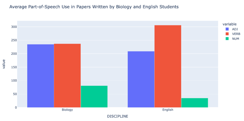
Figure 5: Bar graph showing verb use, adjective use and numeral use, on average, in Biology and English papers
Though admittedly a simple analysis, calculating part-of-speech frequency counts affirms prior studies which posit a correlation between lexico-grammatical features and disciplinary conventions, suggesting this application of spaCy can be adapted to serve other researchers’ corpora and part-of-speech usage queries9.
Fine-Grained Part-of-Speech Analysis
The same type of analysis could be performed using the fine-grained part-of-speech tags; for example, we could look at how Biology and English students use sub-groups of verbs with different frequencies. Fine-grain tagging can be deployed in a similar loop to those above; but instead of retrieving the token.pos_ for each word, we call spaCy to retrieve the token.tag_:
tag_num_list = []
def get_fine_pos_tags(doc):
    dictionary = {}
    num_tag = doc.count_by(spacy.attrs.TAG)
    for k,v in sorted(num_tag.items()):
        dictionary[doc.vocab[k].text] = v
    tag_num_list.append(dictionary)

pos_analysis_df['F_POS'] = pos_analysis_df['Doc'].apply(get_fine_pos_tags)
average_tag_df
Again, we can calculate the amount of times, on average, that each fine-grained part-of-speech appears in Biology versus English paper using the groupby and mean functions.
average_tag_df = tag_counts.groupby(['DISCIPLINE']).mean()

average_tag_df = average_tag_df.round(0)

average_tag_df = average_tag_df.reset_index()

average_tag_df
Now, our DataFrame contains average counts of each fine-grained part-of-speech:
| DISCIPLINE | POS | RB | JJR | NNS | IN | VBG | RBR | RBS | -RRB- | … | FW | LS | WP$ | NFP | AFX | $ | `` | XX | ADD | ’’ | |
|---|---|---|---|---|---|---|---|---|---|---|---|---|---|---|---|---|---|---|---|---|---|
| 0 | Biology | 5.0 | 94.0 | 10.0 | 198.0 | 339.0 | 35.0 | 6.0 | 4.0 | 38.0 | … | 2.0 | 3.0 | 1.0 | 16.0 | 3.0 | 6.0 | 2.0 | 5.0 | 3.0 | 2.0 |
| 1 | English | 35.0 | 138.0 | 7.0 | 141.0 | 414.0 | 50.0 | 6.0 | 3.0 | 25.0 | … | 2.0 | 2.0 | 2.0 | 3.0 | NaN | 1.0 | 3.0 | 5.0 | 3.0 | 5.0 |
spaCy identifies around 50 fine-grained part-of-speech tags, of which ~20 are visible in the DataFrame above. The ellipses in the central column indicates further data which is not shown. Researchers can investigate trends in the average usage of any or all of them. For example, is there a difference in the average usage of past tense versus present tense verbs in English and Biology papers? Three fine-grained tags that could help with this analysis are VBD (past tense verbs), VBP (non third-person singular present tense verbs), and VBZ (third-person singular present tense verbs). Readers may find it useful to review a full list of the fine-grained part-of-speech tags that spaCy generates.
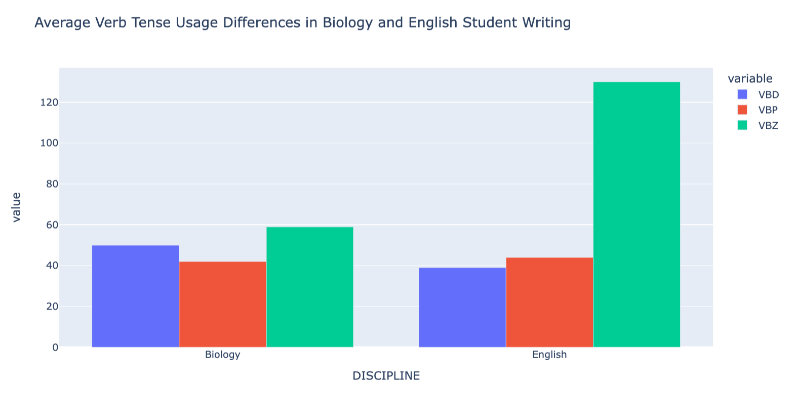
Figure 6: Graph of average usage of three verb types (past tense, third- and non-third person present tense) in English and Biology papers
Graphing these annotations reveals a fairly even distribution of the usage of the three verb types in Biology papers. However, in English papers, an average of 130 third-person singular present tense verbs are used per paper, compared to around 40 of the other two categories. What these differences indicate about the genres is not immediately discernible, but it does indicate spaCy’s value in identifying patterns of linguistic annotations for further exploration by computational and close-reading methods.
The analyses above are only a couple of many possible applications for part-of-speech tagging. Part-of-speech tagging is also useful for research questions about sentence intent: the meaning of a text changes depending on whether the past, present, or infinitive form of a particular verb is used. Equally useful for such tasks as word sense disambiguation and language translation, part-of-speech tagging is additionally a building block of named entity recognition, the focus of the analysis below.
Named Entity Analysis
In this section, you’ll use the named entity tags extracted from spaCy to investigate the second research question: Do students use certain named entities more frequently in different academic genres, and does this signify differences in genre conventions?
To start, we’ll create a new DataFrame with the text filenames, types (genres), and named entity words and tags:
ner_analysis_df = final_paper_df[['Filename','PAPER TYPE', 'Named_Entities', 'NE_Words']]
Using the str.count method, we can get counts of a specific named entity used in each text. Let’s get the counts of the named entities of interest here (PERSON, ORG, DATE, and WORKS_OF_ART) and add them as new columns of the DataFrame.
ner_analysis_df['Named_Entities'] = ner_analysis_df['Named_Entities'].apply(lambda x: ' '.join(x))

person_counts = ner_analysis_df['Named_Entities'].str.count('PERSON')
org_counts = ner_analysis_df['Named_Entities'].str.count('ORG')
date_counts = ner_analysis_df['Named_Entities'].str.count('DATE')
woa_counts = ner_analysis_df['Named_Entities'].str.count('WORK_OF_ART')

ner_counts_df = pd.DataFrame()
ner_counts_df['Genre'] = ner_analysis_df["PAPER TYPE"]
ner_counts_df['PERSON_Counts'] = person_counts
ner_counts_df['ORG_Counts'] = org_counts
ner_counts_df['DATE_Counts'] = date_counts
ner_counts_df['WORK_OF_ART_Counts'] = woa_counts
Reviewing the DataFrame now, our column headings define each paper’s genre and four named entities (PERSON, ORG, DATE, and WORKS_OF_ART) of which spaCy will count usage:
| Genre | PERSON_Counts | LOC_Counts | DATE_Counts | WORK_OF_ART_Counts | |
|---|---|---|---|---|---|
| 0 | Argumentative Essay | 9 | 3 | 20 | 3 |
| 1 | Argumentative Essay | 90 | 13 | 151 | 6 |
| 2 | Argumentative Essay | 0 | 0 | 2 | 2 |
| 3 | Proposal | 11 | 6 | 21 | 4 |
| 4 | Proposal | 44 | 7 | 65 | 3 |
From here, we can compare the average usage of each named entity and plot across paper type.
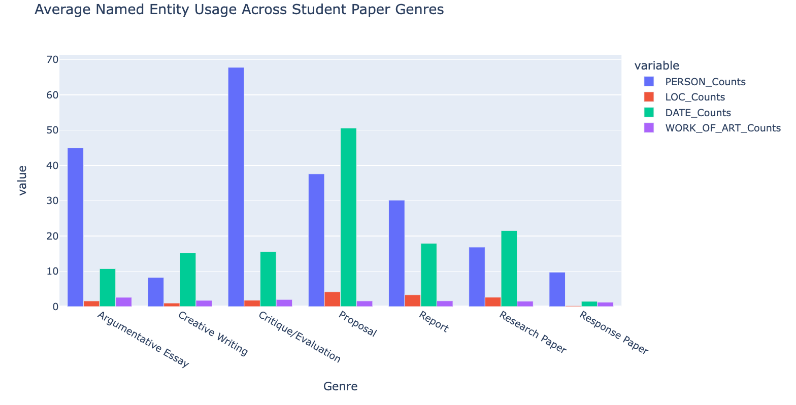
Figure 7: Bar chart depicting average use of Person, Location, Date, and Work of Art named entities across genres
As hypothesized at the start of this lesson: more dates and numbers are used in description-heavy proposals and research papers, while more people and works of art are referenced in arguments and critiques/evaluations. Both of these hypotheses are predicated on engaging with and assessing other scholarship.
Interestingly, people and locations are used the most frequently on average across all genres, likely because these concepts often appear in citations. Overall, locations are most frequently invoked in proposals and reports. Though this should be investigated further through close reading, it does follow that these genres would use locations frequently because they are often grounded in real-world spaces in which events are being reported or imagined.
Analysis of DATE Named Entities
Let’s explore patterns of one of these entities’ usage (DATE) further by retrieving the words most frequently tagged as dates in various genres. You’ll do this by first creating functions to extract the words tagged as date entities in each document and adding the words to a new DataFrame column:
def extract_date_named_entities(doc):
    return [ent for ent in doc.ents if ent.label_ == 'DATE']

ner_analysis_df['Date_Named_Entities'] = final_paper_df['Doc'].apply(extract_date_named_entities)

ner_analysis_df['Date_Named_Entities'] = [', '.join(map(str, l)) for l in ner_analysis_df['Date_Named_Entities']]
Now we can retrieve only the subset of papers that are in the proposal genre, get the top words that have been tagged as “dates” in these papers and append them to a list:
date_word_counts_df = ner_analysis_df[(ner_analysis_df == 'Proposal').any(axis=1)]

date_word_frequencies = date_word_counts_df.Date_Named_Entities.str.split(expand=True).stack().value_counts()
date_word_frequencies[:10]
spaCy outputs a list of the 10 words most-frequently labeled with the DATE named entity tag in Proposal papers:
2004,      24
2003,      18
the        17
2002,      12
2005,      11
1998,      11
2000,       9
year,       9
1977,       8
season,     8
The majority are standard 4-digit dates; though further analysis is certainly needed to confirm, these date entities seem to indicate citation references are occurring. This fits in with our expectations of the proposal genre, which requires references to prior scholarship to justify students’ proposed claims.
Let’s contrast this with the top DATE entities in Critique/Evaluation papers:
# Search for only date words in critique/evaluation papers
date_word_counts_df = ner_analysis_df[(ner_analysis_df == 'Critique/Evaluation').any(axis=1)]

# Count the frequency of each word in these papers and append to list
date_word_frequencies = date_word_counts_df.Date_Named_Entities.str.split(expand=True).stack().value_counts()

# Get top 10 most common words and their frequencies
date_word_frequencies[:10]
Now, spaCy outputs a list of the 10 words most-frequently labeled with the DATE named entity tag in Critique/Evaluation papers:
the         10
winter,      8
years,       6
2009         5
1950,        5
1960,        5
century,     4
decade,      3
of           3
decades,     3
Here, only three of the most-frequently tagged DATE entities are standard 4-digit dates, and the rest are noun references to relative dates or periods. This, too, may indicate genre conventions, such as the need to provide context and/or center an argument in relative space and time in evaluative work. Future research could analyze chains of named entities (and parts-of-speech) to get a better understanding of how these features together indicate larger rhetorical tactics.
Conclusions
Through this lesson, we’ve gleaned more information about the grammatical makeup of a text corpus. Such information can be valuable to researchers who are seeking to understand differences between texts in their corpus: What types of named entities are most common across the corpus? How frequently are certain words used as nouns versus objects within individual texts and corpora? What may these frequencies reveal about the content or themes of the texts themselves?
While we’ve covered the basics of spaCy in this lesson, it has other capacities, such as word vectorization and custom rule-based tagging, that are certainly worth exploring in more detail. This lesson’s code can also be altered to work with custom feature sets. A great example of working with custom feaature sets is Susan Grunewald’s and Andrew Janco’s lesson, Finding Places in Text with the World Historical Gazetteer, in which spaCy is leveraged to identify place names of German prisoner of war camps in World War II memoirs, drawing on a historical gazetteer of camp names.
spaCy is an equally helpful tool to explore texts without fully-formed research questions in mind. Exploring linguistic annotations can propel further research questions and guide the development of text-mining methods.
Ultimately, this lesson has provided a foundation for corpus analysis with spaCy. Whether you wish to investigate language use in student papers, novels, or another large collection of texts, this code can be repurposed for your use.
Endnotes
-
Matthew Brook O’Donnell and Ute Römer, “From student hard drive to web corpus (part 2): The annotation and online distribution of the Michigan Corpus of Upper-level Student Papers (MICUSP),” Corpora 7, no. 1 (2012): 1–18. https://doi.org/10.3366/cor.2012.0015. ↩
-
Jack Hardy and Ute Römer, “Revealing disciplinary variation in student writing: A multi-dimensional analysis of the Michigan Corpus of Upper-level Student Papers (MICUSP),” Corpora 8, no. 2 (2013): 183–207. https://doi.org/10.3366/cor.2013.0040. ↩
-
Laura Aull, “Linguistic Markers of Stance and Genre in Upper-Level Student Writing,” Written Communication 36, no. 2 (2019): 267–295. https://doi.org/10.1177/0741088318819472. ↩
-
Sugene Kim, “‘Two rules are at play when it comes to none ’: A corpus-based analysis of singular versus plural none: Most grammar books say that the number of the indefinite pronoun none depends on formality level; corpus findings show otherwise,” English Today 34, no. 3 (2018): 50–56. https://doi.org/10.1017/S0266078417000554. ↩
-
Carol Berkenkotter and Thomas Huckin, Genre knowledge in disciplinary communication: Cognition/culture/power, (Lawrence Erlbaum Associates, Inc., 1995). ↩
-
Jack Hardy and Eric Friginal, “Genre variation in student writing: A multi-dimensional analysis,” Journal of English for Academic Purposes 22 (2016): 119-131. https://doi.org/10.1016/j.jeap.2016.03.002. ↩
-
Alexandra Schofield, Måns Magnusson and David Mimno, “Pulling Out the Stops: Rethinking Stopword Removal for Topic Models,” Proceedings of the 15th Conference of the European Chapter of the Association for Computational Linguistics 2 (2017): 432-436. https://aclanthology.org/E17-2069. ↩
-
Fiona Martin and Mark Johnson. “More Efficient Topic Modelling Through a Noun Only Approach,” Proceedings of the Australasian Language Technology Association Workshop (2015): 111–115. https://aclanthology.org/U15-1013. ↩
-
Jack Hardy and Ute Römer, “Revealing disciplinary variation in student writing: A multi-dimensional analysis of the Michigan Corpus of Upper-level Student Papers (MICUSP),” Corpora 8, no. 2 (2013): 183–207. https://doi.org/10.3366/cor.2013.0040. ↩