A Table of Contents
Contents
- A Table of Contents
1. Lesson Overview
Researchers often need to be able to search a corpus of texts for a defined list of terms. In many cases, historians are interested in certain places named in a text or texts. This lesson details how to programmatically search documents for a list of terms, including place names. To begin, we will produce a tab-separated value (TSV) file where each row gives the matched term and the term’s location in the text. We also generate a visualization that can be used to interpret the matches in context and to assess their usefulness for a given project. The goal of the lesson is to systematically search a text corpus for place names and then to use a service to locate and map historic place names. This lesson will be useful for anyone wishing to perform named entity recognition (NER) on a text corpus. Other users may wish to skip the text extraction portion of this lesson and focus solely on the spatial elements of the lesson, that is gazetteer building and using the World Historical Gazetteer (WHG). These spatial steps are especially useful for someone looking to create maps depicting historical information in a largely point and click interface. We have designed this lesson to show how to combine text analysis with mapping, but understand that some readers may only be interested in one of these two methodologies. We urge you to try both parts of the lesson together if you have time, as this will enable you to learn how text analysis and mapping can be combined in one project. Additionally, it will demonstrate how the results of these two activities can be ported into another form of digital analysis.
In this lesson, readers will use the Python pathlib library to load a directory of text files. For those with an existing gazetteer or list of terms, readers will then be able to create a list of term matches and their locations in a text. Those without a gazetteer, can use a statistical language model to identify places. Users will create a TSV file in the Linked Places Format, which can then be uploaded to the World Historical Gazetteer. Linked Places Format is designed to standardize descriptions of places and is primarily intended to link gazetteer datasets. It is a form of Linked Open Data (LOD), which attempts to make datasets interoperable. Once a user uploads their Linked Places Format dataset to the WHG, they can use the WHG for reconciliation and geocoding. Reconciliation is the alignment of a user’s dataset with the index of place records in the WHG. This is what enables the WHG to geocode, or ‘match’, a place’s name with its geographic coordinates. These geographic coordinates are what allow a list of names to be transformed into plots on a map.
Please note that the sample data and context of this lesson constitute an example of multilingual digital humanities. The memoir texts are in German, while the list of place names represent German transliterations of Russian names for places across the former Soviet Union circa 1941-56.
2. Historical example
This lesson applies co-author Susan Grunewald’s research and serves to demonstrate how her practical methods can be beneficial to historians. Grunewald mapped forced labor camps where German Prisoners of War (POWs) were held in the former Soviet Union during and after the Second World War. Her maps have been used to argue that contrary to popular memory, German POWs in the Soviet Union were sent more commonly to industrial and reconstruction projects in Western Russia rather than Siberia. Grunewald’s research went on to investigate whether POW memoirs gave a misrepresentation of Siberian captivity, which could have helped to create or promulgate this popular memory.
In this lesson, we will use a list of camp names to identify mentions of particular camps and their locations in POW memoirs. This data can then be mapped to demonstrate Grunswald’s thesis that not all direct mentions of places in POW memoirs were in Siberia.
3. Building a corpus
To facilitate this lesson, we have compiled a sample dataset of selections from digitized POW memoirs to search for place names. Due to copyright restrictions, the dataset does not include the full text of the memoirs but rather snippets from roughly 35 sources. We have provided a sample textual corpus for download.
Alternatively, to build your own corpus for this exercise, all you need are files saved in .txt format. If you need help building a corpus of .txt files, you may find this Programming Historian tutorial by Andrew Akhlaghi useful — it provides instructions for transforming PDF files into machine readable text files.
4. Building a gazetteer
A gazetteer is an index or directory of place names. For our example, we are using information from an encyclopedia about German prisoners of war camps catalogued in central Soviet government documents. This particular encyclopedia lists the nearest location (e.g., settlement or city) for each of the roughly 4,000 forced labor POW camps.
As a quick side note, this encyclopedia is an interesting example of the many layers of languages involved when studying Soviet history. The original source book is in German, meaning it uses German transliteration standards for the Russian Cyrillic alphabet. Generally, the places named in the book represent the Russified Soviet names. This means that the places listed may not be named as we know them today. Many are Russified versions of places that are now more commonly known by different names due to post-Soviet identity politics. Some of the places do still have the same name, but an added complexity is that the German transliteration we read here, is from a Russian transliteration of a local language, such as Armenian. As we proceed with the mapping process, it is important we remain aware of these extra layers of possible distortion.
The directory of place names we use in this lesson is an example of a historical gazetteer. That is, these names are those utilized by a particular regime during a specific historical context. Trying to map the places mentioned in the memoirs is therefore not a simple task as the names have changed both in the Soviet and post-Soviet era. By using a resource such as the World Historical Gazetteer, it is possible to use the larger historical gazetteer system as a crosswalk between the historical and contemporary names. This gives us the ability to map the locations on a modern map. This process is not straightforward if you are working with larger, more common geographic information systems such as Google Maps or ArcGIS. The WHG is not perfect, though. It works well for matching historical place names with modern ones only when those links already exist in the gazetteer, which is continuously growing due to active user contributions. However, certain place names are not currently supported – sometimes because the links between the historical and contemporary names are not yet established, or because their locations are unknown.
Users can build their own gazetteer simply by listing places of importance for their study in an Excel spreadsheet and saving the document as a comma-separated value (CSV) file. Note that for this lesson, and whenever working with the World Historical Gazetteer, it is best to focus on the names of settlements (i.e., towns and cities). This is because the World Historical Gazetteer does not currently support mapping and geolocating of states or countries.
We have provided a sample gazetteer of German names for prisoner of war camps for use with this lesson.
5. Finding Places in Text with Python
From your computer’s perspective, text is nothing more than a sequence of characters. If you ask Python to iterate a snippet of text, you’ll notice that it returns just one letter at a time. Note that the index starts at 0, not 1, and that spaces are part of the sequence.
text = "Siberia has many rivers."
for index, char in enumerate(text):
    print(index, char)
0  S
1  i
2  b
3  e
4  r
5  i
6  a
7
8  h
9  a
10 s
11
12 m
13 a
14 n
15 y
16
17 r
18 i
19 v
20 e
21 r
22 s
23 .
When we ask Python to find the word “rivers,” in a larger text, it is specifically searching for a lower-case “r” followed by “i” “v” and so on. It returns a match only if it finds exactly the right letters in the right order. When it makes a match, Python’s .find() function will return the location of the first character in the sequence. For example:
text = "Siberia has many rivers."
text.find("rivers")
17
Keep in mind that computers are very precise and picky. Any messiness in the text will cause the word to be missed, so text.find("Rivers") returns -1, which means that the sequence “Rivers” (with an uppercase R) could not be found. You can also inadvertently match characters that are part of the sequence, but don’t represent a whole word. Try text.find("y riv"). You retrieve 15 matches because that is part of the “y riv” sequence. So while it is present in the text, this isn’t a term that you’d normally set out to find.
6. Natural language processing
While pure Python is sufficient for many tasks, natural language processing (NLP) libraries allow us to work computationally with the text as language. NLP reveals a whole host of linguistic attributes of the text that can be used for analysis. For example, it can identify if a word is a noun or a verb using ‘part of speech’ tagging. We can also use NLP to identify the direct object of a verb, to determine who is speaking and locate the subject of that speech. NLP provides your programs with additional information which can open up new forms of analysis. As historians, we can also appreciate how NLP prompts us to consider the linguistic aspects of our sources in ways that we might otherwise not.
Our first NLP task is tokenization. This is where our text is split into meaningful parts, known as word tokens. The sentence, “Siberia has many rivers.” can be split into the tokens: <Siberia><has><many><rivers><.>. Note that the closing punctuation is now distinct from the word rivers. The rules for tokenization depend on the language you are using. For English and other languages that use spaces between words, you often achieve good results simply by splitting the tokens where there are spaces. However, more specific rules are needed to separate punctuation from a token, to split and normalize elided words (for example, “Let’s” > Let us) as well as other exceptions that don’t follow regular patterns.
For this lesson, we’ll be using an NLP library called spaCy. This library focuses on “practical NLP” and is designed to be fast and simple so that it works well on a basic laptop. For these reasons, spaCy can be a good choice for historical research tasks. As a library, spaCy is opinionated and its simplicity comes at the cost of choices being made on your behalf. For those who are new to NLP, the spaCy documentation is a good place to learn about how their design choices influence the way the software operates, and will help you to assess whether spaCy is the best solution for your particular project. That said, spaCy works extremely well for tasks such as tokenization, part-of-speech tagging and named entity recognition. Similar libraries, such as NLTK, CLTK or Stanza are also excellent choices and you can learn a lot by comparing the different approaches these libraries take to similar problems.
Once you’ve run pip install spacy (see the Programming Historian article “Installing Python Modules with pip” by Fred Gibbs if you’re new to pip), you will be able to import the ‘object’ for your language so that the tokenization rules are specific to your language. The spaCy documentation lists the currently supported languages and their language codes.
To load a new language, you will import it. For example, from spacy.lang.de import German or from spacy.lang.en import English
In Python, this command navigates to spaCy’s directory, then into the subfolders lang and de to import the Language object called German from that folder.
We are now able to tokenize our text with the following:
from spacy.lang.de import German
nlp = German()
doc = nlp("Berlin ist eine Stadt in Deutschland.")
for token in doc:
    print(token.i, token.text)
0 Berlin
1 ist
2 eine
3 Stadt
4 in
5 Deutschland
6 .
Note that each token now has its own index number.
With the language object we can tokenize the text, remove ‘stop words’ (words to be filtered out before processing) and punctuation, and many other common text processing tasks. For further information, Ines Montani has created an excellent free online course (available in English and six other languages).
6.1 Load the gazetteer
Now let’s focus back on the task at hand. We need to load our list of place names and find where they occur in a text. To do this, let’s start by reading the file containing our list of names. We’ll use Python’s pathlib library, which offers a simple way to read the text or data in a file. In the following example, we will import pathlib and use it to open a file called ‘gazetteer.txt’ and load its text. We then create a Python list of the place names by splitting on the new line character “\n”. This assumes that your file is structured with a new line for each place name. If you’ve used a different format in your file, you may need to split on the comma “,” or tab ”\t”. To do this, just change the value inside .split() below.
from pathlib import Path

gazetteer = Path("gazetteer.txt").read_text('utf8')
gazetteer = gazetteer.split("\n")
At this point, you should be able to print(gazetteer) and get a nice list of places:
print(gazetteer)
['Armenien', 'Aserbaidshan', 'Aserbaidshen', 'Estland', … ]
6.2 Matching Place Names
Now that we have a list of place names, let’s find where those terms appear in our texts. As an example, let’s use this sentence:
Karl-Heinz Quade ist von März 1944 bis August 1948 im Lager 150 in Grjasowez interniert.
“Karl-Heinz Quade was interned in Camp 150 in Gryazovets from March 1944 to August 1948.” There’s one place name in this sentence, Gryazovets, which is a town 450 km from Moscow. We just need to show our computer how to find it (and all the other places we care about). To do this, we’ll use spaCy’s Matcher tool, which is a powerful tool for searching the tokenized text for patterns in words and their attributes.
from spacy.lang.de import German
from spacy.matcher import Matcher

nlp = German()

doc = nlp("Karl-Heinz Quade ist von März 1944 bis August 1948 im Lager 150 in Grjasowez interniert.")

matcher = Matcher(nlp.vocab)
for place in gazetteer:
    pattern = [{'LOWER': place.lower()}]
    matcher.add(place, [pattern])

matches = matcher(doc)
for match_id, start, end in matches:
    print(start, end, doc[start:end].text)
13 14 Grjasowez
The Matcher will find tokens that match the patterns that we’ve given it. Note that we’ve changed the place names to be written in all lower case letters so that the search will be case-insensitive. Use “ORTH” instead of ”LOWER” if you want to perform a case-sensitive search. Note that we retrieve a list including exact matches as well as the start and end indexes of the matched spans or tokens. With Matchers, we are able to search for combinations of more than one word such as “New York City” or “Steamboat Springs.” This is really important because you might have “York”, “New York” and “New York City” in your places list.
If you’ve ever worked with regular expressions, some of this may feel familiar. However, rather than matching on sequences of characters, here we’re matching token patterns that can also include parts of speech and other linguistic attributes of a text. As an example, let’s also match on “Camp 150” (which is “Lager 150” in German). We’ll add a new pattern that will identify a match whenever we have “Lager” followed by a number.
pattern = [{'LOWER': 'lager'},  #the first token should be ‘lager’
           {'LIKE_NUM': True}] # the second token should be a number

# Add the pattern to the matcher
matcher.add("LAGER_PATTERN", [pattern])
We now see (start index, end index, match):
10 12 Lager 150
13 14 Grjasowez
The pattern can be any sequence of tokens and their attributes. For more on how to wield this new superpower, see the spaCy Matcher documentation, the spaCy course and the Rule-based Matcher Explorer.
6.3 Loading Text Files
In the examples above, we processed a single sentence. That might be all you need, but most often you’ll need to process multiple texts at once. The code below will load an entire directory full of .txt files. Pathlib gives us an easy way to iterate over all the files in the directory using iterdir() as well as a read_text() method that will load the text. The code below will generate a list of the filename, location and name of every place from our gazetteer that appears in the texts.
for file in Path('folder_with_texts_in_it').iterdir():
    doc = nlp(file.read_text())
    matches = matcher(doc)
    for match_id, start, end in matches:
        print(file.name, start, end, doc[start:end].text)
6.4 Term Frequency
At this point you may want to know which items appear most frequently in the text. To count frequencies, you can use Python’s Counter object. In the following cell, we create an empty list and then add the text for each match. The counter will then return the frequency for each term in the list.
from collections import Counter

count_list = []
for match_id, start, end in matches:
    count_list.append(doc[start:end].text)

counter = Counter(count_list)

for term, count in counter.most_common(10):
    print(term,count)
Lager 150 1
Grjasowez 1
6.5 Named Entity Recognition
Up to this point, we have been using the spaCy Matcher to search a document for specific place names. It will find any of the places in our list that occur in the text. However, what if we want to find places including those not in our list? Can we retrieve all the place names that appear in the text? For this task, there are pre-trained models available in many languages for identifying place names. These are statistical models that have learned the general “look and feel” of place names and can make predictions. This enables the model to identify place names even if they were not included in its training data. But it also means that the model can make mistakes. With the jump into machine learning, it’s important that you keep in mind that the machine is making informed predictions based on what it has learned. If your materials are significantly different from what the model was trained on, say Ottoman government texts rather than contemporary Turkish newspaper articles, you should expect rather poor performance. However, it is also possible to fine-tune a model using your materials to improve accuracy.
To work with a pre-trained model in spaCy, you’ll need to download one. A list of the current options can be found in the spaCy documentation. For our German example, use the command-line interface to download the small model trained on newspaper articles: python -m spacy download de_core_news_sm. To load the model and identify named entities, use the following:
import spacy
nlp = spacy.load("de_core_news_sm")

doc = nlp("Karl-Heinz Quade ist von März 1944 bis August 1948 im Lager 150 in Grjasowez interniert.")
for ent in doc.ents:
    print(ent.text, ent.label_, ent.start, ent.end)
Karl-Heinz Quade PER 0 2
Grjasowez LOC 13 14
Just by looking at the text and the relationships between words, the model is able to correctly identify that Karl-Heinz Quade is a person (PER) and that Grjasowez is a place (LOC). Named entity recognition is a powerful tool for finding places, people and organizations in text. However, you are likely to encounter machine errors, so it’s important to review the results and to correct errors. With Matcher, you won’t encounter these mistakes, but you also won’t find place names that are not featured in the gazetteer.
6.6 DisplaCy
To see your results in the context of the text, spaCy includes a useful tool called displaCy. displaCy will display an image of the text alongside any predictions made, which can be very useful when assessing whether the results are going to be helpful to your research or introduce too many machine errors to be practical. spaCy also offers a web application that enables you to assess predictions quickly. Visualizations can be created either using a Python script or by running a Jupyter notebook.
python script
from spacy import displacy
displacy.serve(doc, style="ent")

Figure 1: entity recognition image
jupyter notebook
displacy.render(doc, jupyter=True, style="ent")
With statistical models, you can also use displaCy to create a useful visualization of the relationships between words in the text. Just use style='dep' to generate this form of visualization.
displacy.render(doc, jupyter=True, style="dep")

Figure 2: dependency visualization
DisplaCy visualizations can also be saved to a file for use elsewhere (spaCy’s documentation provides further guidance).
from pathlib import Path

svg = displacy.render(doc, style="dep")
output_path = Path("sentence.svg")
output_path.write_text(svg)
6.7 Named Entity Linking
While it’s useful to note that Karl-Heinz Quade is a person, it would be even better to know who Karl-Heinz Quade is. Named entity linking is the process of connecting a place or person’s name to a specific record in a knowledge base. This link connects the predicted entity to a unique record and its associated data. For example, DBpedia records for places often contain data including the latitude and longitude, region, country, time zone, and population. By connecting our text to the DBpedia knowledge base, we are able to utilize external information in our analysis.
There is a useful Python library for spaCy known as the DBpedia Spotlight which can attempt to match predicted entities with records in DBpedia. This relationship will then be visible as part of the ‘entity span’ annotation. To install the DBpedia Spotlight library, enter pip install spacy-dbpedia-spotlight in the command line and press enter.
import spacy
nlp = spacy.load('de_core_news_sm')
nlp.add_pipe('dbpedia_spotlight', config={'language_code': 'de'})

doc = nlp("Karl-Heinz Quade ist von März 1944 bis August 1948 im Lager 150 in Grjasowez interniert.")
for ent in doc.ents:
    print(ent.text, ent.label_, ent.kb_id_)
Grjasowez DBPEDIA_ENT http://de.dbpedia.org/resource/Grjasowez
interniert DBPEDIA_ENT http://de.dbpedia.org/resource/Internierung
Note that we now have entities in the document with the “DBPEDIA_ENT” label and the URI for the DBpedia record. Karl-Heinz Quade does not feature in DBpedia, so we don’t get a match, but the Grjasowez record has a wealth of information. To access the associated data, you can send a request to the DBpedia server. Note that we have replaced the human-readable page “resource” with the machine-readable operator “data”. We then add “.json” to the record name, which will return the data as JSON. We can use the requests library to parse the JSON data and make it ready for use in our Python script.
import requests
data = requests.get("http://de.dbpedia.org/data/Grjasowez.json").json()
You can explore this data using print(data) or data.keys(). For more on JSON, see Matthew Lincoln’s lesson for the Programming Historian.
Here is an example of how to access the latitude and longitude for this particular result:
data['http://de.dbpedia.org/resource/Grjasowez']['http://www.georss.org/georss/point'][0]['value']
'58.88333333333333 40.25'
Before moving on, it is important to note that spacy-dbpedia-spotlight is similar to the Matcher. It takes a predicted entity (a person, place, or organization) and searches DBpedia for a corresponding entry. It can identify a match, but it is not able to look at the context of the text to predict whether “I. Ivanov” is the famous Bulgarian badminton player or the Russian skier. Whereas, spaCy has the capacity to use the surrounding text to disambiguate the results. “Ivan cherished badminton” and “The great skier, Ivanov…” will return different link predictions given the textual context and frequency of the record in the corpus. This is a more involved process than we can detail within the scope of this lesson. However, one of the developers of spaCy, Sofie Van Landeghem, has recorded a very useful video on this process for those advanced users who require this functionality.
6.8 Export Our Data
The final step in this section is to export our Matches in the tab separated value (TSV) format required by the World Historical Gazetteer. If you’ve used a spreadsheet program like Excel or Google Sheets, then you will already be familiar with tabular data. This is information structured in rows and columns. To store tabular data in a simple format, programmers often use tab-separated value (TSV) files. These are simple text files including symbols that split the text into rows and columns. Rows are separated by the new line character \n and rows are split into columns by tabs \t.
start_date = "1800" #YYYY-MM-DD
end_date = "2000"
source_title = "Karl-Heinz Quade Diary"

output_text = ""
column_header = "id\ttitle\ttitle_source\tstart\tend\n"
output_text += column_header

places_list = []
if matches:
    places_list.extend([ doc[start:end].text for match_id, start, end in matches ])
if doc.ents:
    places_list.extend([ ent.text for ent in doc.ents if ent.label_ == "GPE" or ent.label_ == "LOC"])

# remove duplicate place names by creating a list of names and then converting the list to a set
unique_places = set(places_list)

for id, place in enumerate(unique_places):
    output_text += f"{id}\t{place}\t{source_title}\t{start_date}\t{end_date}\n"

filename = source_title.lower().replace(' ','_') + '.tsv'
Path(filename).write_text(output_text)
print('created: ', filename)
7. Uploading to the World Historical Gazetteer
Now that we have a Linked Places TSV, we will upload it to the World Historical Gazetteer (WHG). The WHG is a fully web-based application. It indexes place names drawn from historical sources, adding temporal depth to a corpus of approximately 1.8 million modern records. This is especially useful for places which have changed names over time. By using the WHG, users can upload their data and rapidly find the coordinates of historical places (provided that the places are in the WHG index and have coordinates). As mentioned in the gazetteer section above, this service provides automatic geocoding that is suitable for use with historical data. Many common geocoding services including Google Maps, as well as those behind a paywall barrier such as ArcGIS, are unsuitable for historical research as they are based primarily upon 21st century information. They rarely support historical place name information beyond the most common instances. Additionally, the WHG also supports a multitude of languages. Finally, geocoding and basic mapping are achievable through a graphical user interface. This circumnavigates the need to use a script, to trace layers from maps in a different program, or create relational databases and table joins in GIS software.
The WHG is free to use. To get started, register for an account and then sign in.
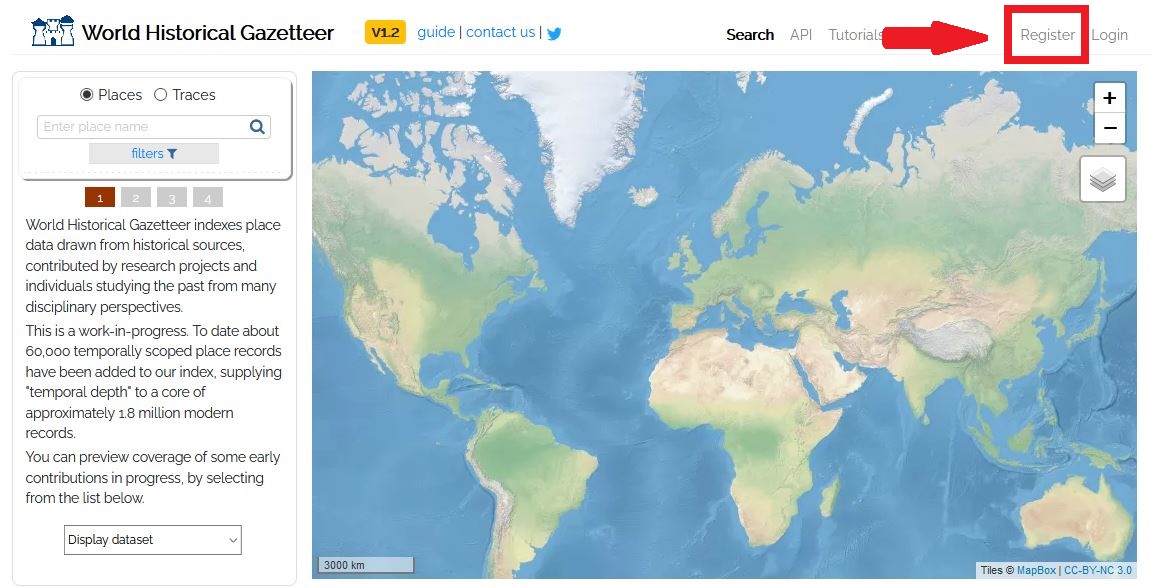
Figure 3: Register
After registering and logging in, you will be taken to the “Datasets” tab. Press “add new” to upload your Linked Pasts TSV to the WHG.
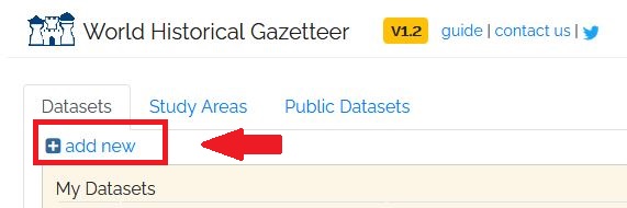
Figure 4: Add Data
Insert a title, such as “POW Memoir Places,” and add a brief description. Do not check the public box for now, as we do not want this dataset to be visible to anyone but your own user account. If you want to contribute to the WHG, you can upload your historic place name information and adjust the privacy settings in the future. Next, browse your computer to locate your Linked Places TSV file and upload it. Do not change the formatting selection - Delimited/Spreadsheet must remain selected. The image below shows a properly formatted upload dialogue box.
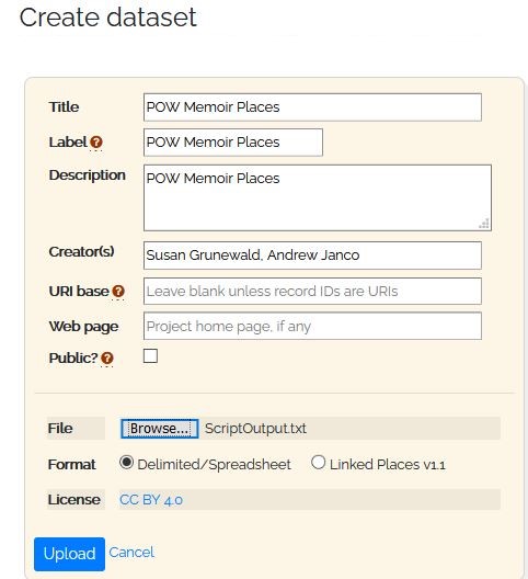
Figure 5: Adding Data
Once the dataset is successfully uploaded, you can begin what is known as the reconciliation process. Back on the “Datasets” tab, click on the TSV file you’ve uploaded. This will take you to a new screen to preview the dataset’s metadata. Click on the “Reconciliation” tab at the top of this page. Reconciliation is the process of entries in your TSV file to the database of place names and their additional relations in the WHG. On the “Reconciliation” tab, press the “add new task” button.
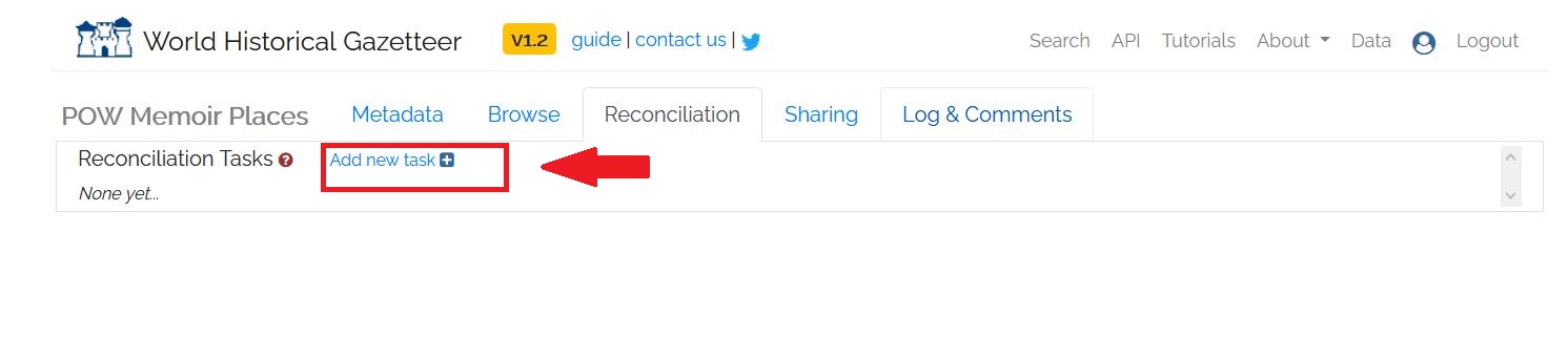
Figure 6: Starting Reconciliation Part 1
You currently have the option to reconcile your data with Getty TGN or Wikidata. Select Wikidata and press start. If you want to limit the geographical area of your results, apply a geographic constraint filter before pressing start. If none of the pre-defined regions are acceptable, you can create your own user area to fine-tune the results retrieved in the reconciliation process.
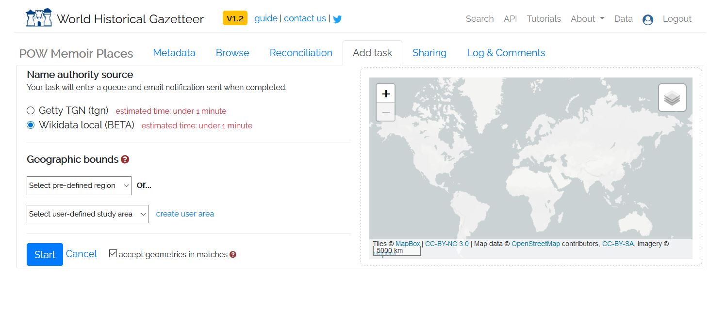
Figure 7: Starting Reconciliation Part 2
After pressing Start, you will be returned to the main “Reconciliation” tab. The process will run for a while and you will receive an email when the process is complete. You can also refresh the screen every few seconds to see if it is done. When the reconciliation is complete, you will be advised how many results need to be reviewed for each ‘Pass’ of the process. In this case we reconciled 133 records, of which 126 were’ hits’. We now have to do a manual review of the ‘hits’ to see if they are correct Matches. Press the “Review” button next to “Pass 1” to begin.
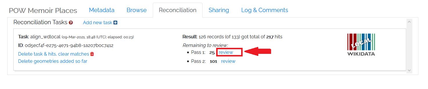
Figure 8: Starting Reconciliation Part 3
You will be taken to a new screen that asks you to match the place names in your TSV file with records in the WHG. You will be given a choice of potential matches on the right hand side of the screen. Hover over them and they will appear as green flashes on the map illustration screen. Your options are “closeMatch” or “no match”. You can only have one closeMatch per place so choose the one from the reconciliation area that best describes your place in question. It is also possible that none of the suggested matches are correct, and in that case select “no match”.
The more information you put into the LP-TSV format, such as country codes, the easier it will be to make these matches. The associated information from the LP-TSV upload will appear on the left hand side of the reconciliation screen to help you understand all of the information provided on the right hand side. If you are building your own dataset, it is worth taking the time to add a country codes (ccodes) column into the file you upload as well as a type column with the corresponding type (e.g. settlement, state, country).
Given the bare-bones nature of this upload, it will be a little harder to reconcile these matches. All of the results should originate from the countries that made up the former Soviet Union: Russia, Ukraine, Belarus, Estonia, Latvia, Lithuania, Moldova, Armenia, Azerbaijan, Georgia, Uzbekistan, Kazakhstan, Kyrgyzstan, Tajikistan, and Turkmenistan. To see this in action, let’s start the reconciliation process. Our first review is for Jelabuga. It is indeed a close match for Yelabuga, which we note is a variant of Yelabuga being listed as “Jelabuga@de,” confirming that Jelabuga is the German language variant of Yelabuga. We will select “closeMatch” and then “save,” which will advance us to the next item for review.
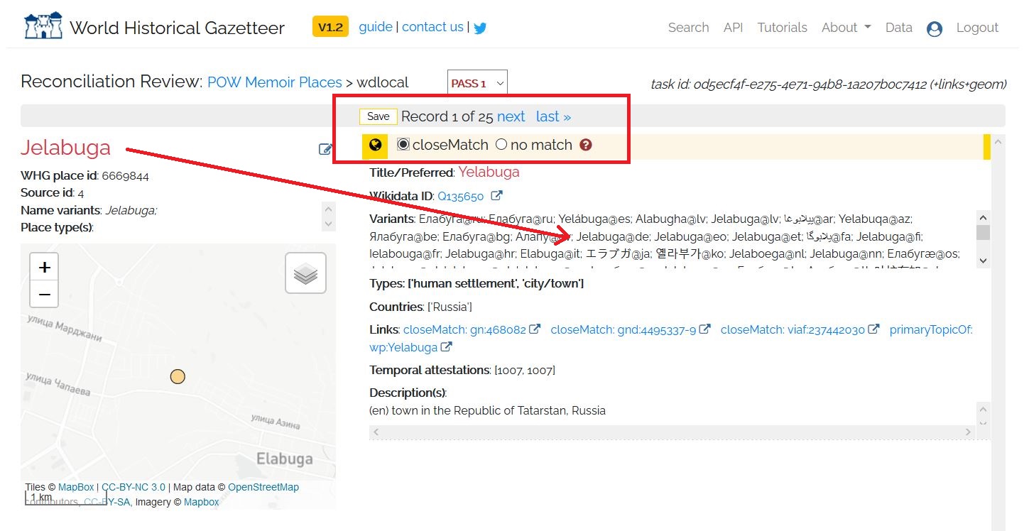
Figure 9: closeMatch
The next location for review is Keller. We can tell that this example is “no match” because the suggested match is a place in Italy. As our data only concerns places in the former Soviet Union, we can save “no match” and quickly move on. Note that if you realize you’ve made a mistake, you can go back one previous save by pressing the “Undo last save” button on the top left of the “Reconciliation Review” screen.
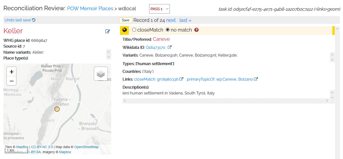
Figure 10: No Match
Go ahead and finish the review of the remaining 23 records for Pass 1. As a hint, of the 25 places for Pass 1 reconciliation, only Yelabuga, Kupjansk, Atkarsk, Makejewka, Kokand, Selenodolsk, Merefa, Usa (in Belarus), Wjasma, Fastow, and Owrutsch are close matches.
Once you complete review of Pass 1, you are automatically taken to complete the review of Pass 2. For now, go back to the Data button on the top right corner of the screen to return to your data tab. Click on your “POW Memoir Places” dataset again to go to its metadata page. If you click on the “Browse” tab next to the “Metadata” tab, you will now see that there are geometries for the places we decided were close matches. These places now appear on the map preview.
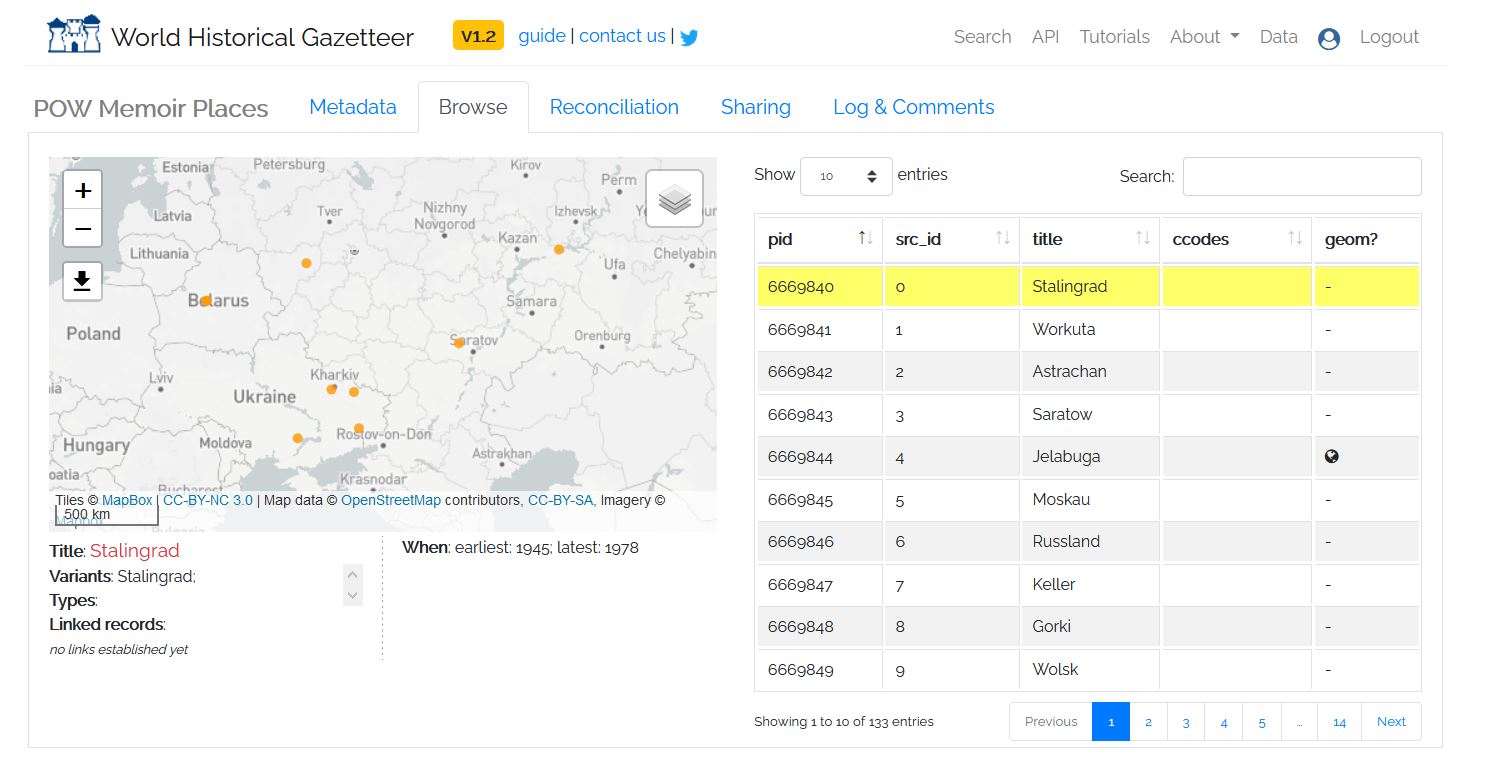
Figure 11: Map Preview
If you click on the “Reconciliation” tab again, you can click on review next two Pass 2 to keep reviewing locations. If you wish, you can continue going through the 101 locations for Pass 2. Should you complete the review process, you will produce a map that looks like the one below.
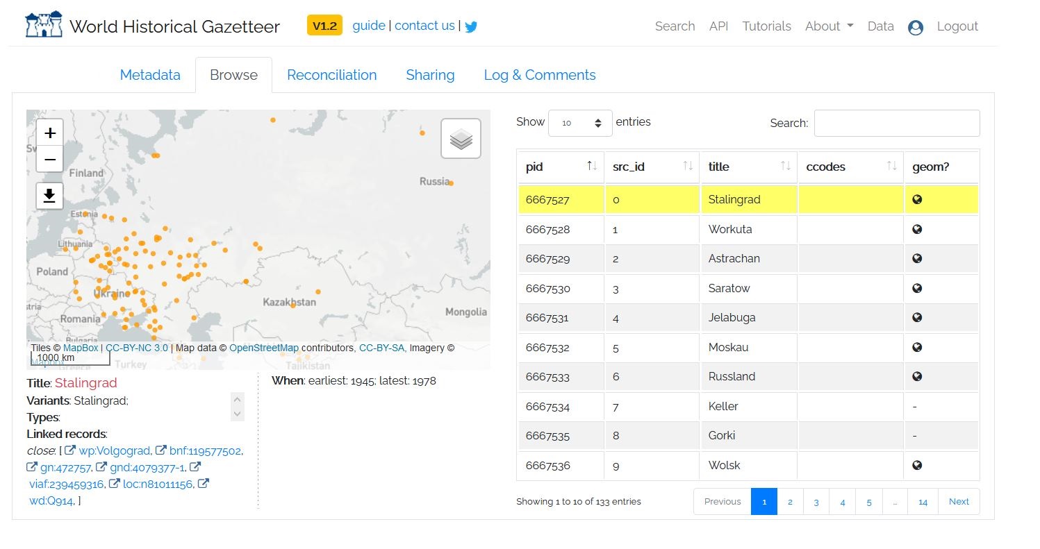
Figure 12: Full Map
If you wish to download an image file of the map, you can do so by hovering over the download symbol in the top left corner of the map preview and then sliding your mouse over to the arrows that appear showing “download current size.”
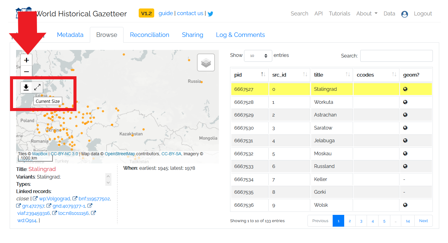
Figure 13: Map Download
8. Future Mapping Work and Suggested Further Lessons
The reconciliation process will not only give you a static map, but it will also give you an augmented dataset to download. This augmented file will include the latitude and longitude coordinates for your close matches. You can download the augmented file from the dataset’s Metadata tab. In the bottom right hand corner, there is a box labelled “Downloads” and you can choose either the Linked Placed format GeoJSON file or a TSV.
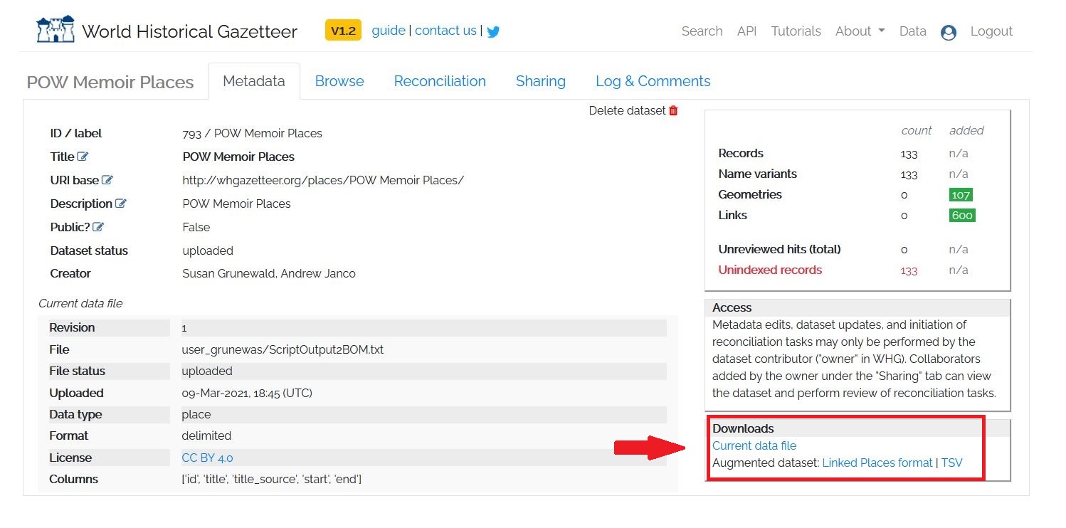
Figure 14: Augmented Data
You can then use the augmented dataset in desktop or web-based mapping applications such as QGIS or ArcGIS Online to undertake more advanced geographic information system (GIS) spatial analysis. In these programs, you can change the map visualizations, perform analysis, or make a multimedia web mapping project. We highly recommend you look at the additional Programming Historian mapping lessons, specifically Installing QGIS and Adding Layers as well as Creating Vector Layers in QGIS to see how you can use the results of this lesson to carry out further analysis.
