Contents
Lesson Goals
In this lesson you will learn how to create vector layers based on scanned historical maps. In Intro to Google Maps and Google Earth you used vector layers and created attributes in Google Earth. We will be doing the same thing in this lesson, albeit at a more advanced level, using QGIS software.
Vector layers are, along with raster layers, one of the two basic types of data structures that store data. Vector layers use the three basic GIS features – lines, points, and polygons – to represent real-world features in digital format. Points can be used to represent specific locations, such as towns, buildings, events, etc. (the scale of your map will determine what you represent as a point – in a map of a province, a town would be a point, whereas in a map of a town, a building might be a point). Lines can effectively represent features such as roads, canals, railways, and so on. Polygons (effectively enclosed shapes with more than a few sides) are used to represent more complex objects such as the boundaries of a lake, country, or electoral riding (again, scale will affect your choice – large buildings in a close-up map of a city might be better represented as polygons than as points).
In this lesson you will be creating shapefiles (which are a type of vector data) to represent the historical development of communities and roads in Prince Edward Island. Each shapefile can be created as one of the three types of features: line, point, polygon (though these features can’t be mixed within a shapefile) . Each feature you create in a shapefile has a corresponding set of attributes, which are stored in an attribute table. You will create features and learn how to modify them, which involves not only the visual creation of the three types of features, but also the modification of their attributes. To do so, we will use the files from Installing QGIS 2.0 and Adding Layers concerning Prince Edward Island.
Getting Started
Start by downloading the PEI_Holland map to the project folder:
Open the file you saved at the end of Installing QGIS 2.0 and Adding Layers. You should have the following layers in your Layers window:
- PEI_placenames
- PEI_highway
- PEI HYDRONETWORK
- 1935 inventory_region
- coastline_polygon
- PEI-CumminsMap1927
Uncheck all of these layer except for PEI_placenames, coastline_polygon and PEI_CumminsMap1927
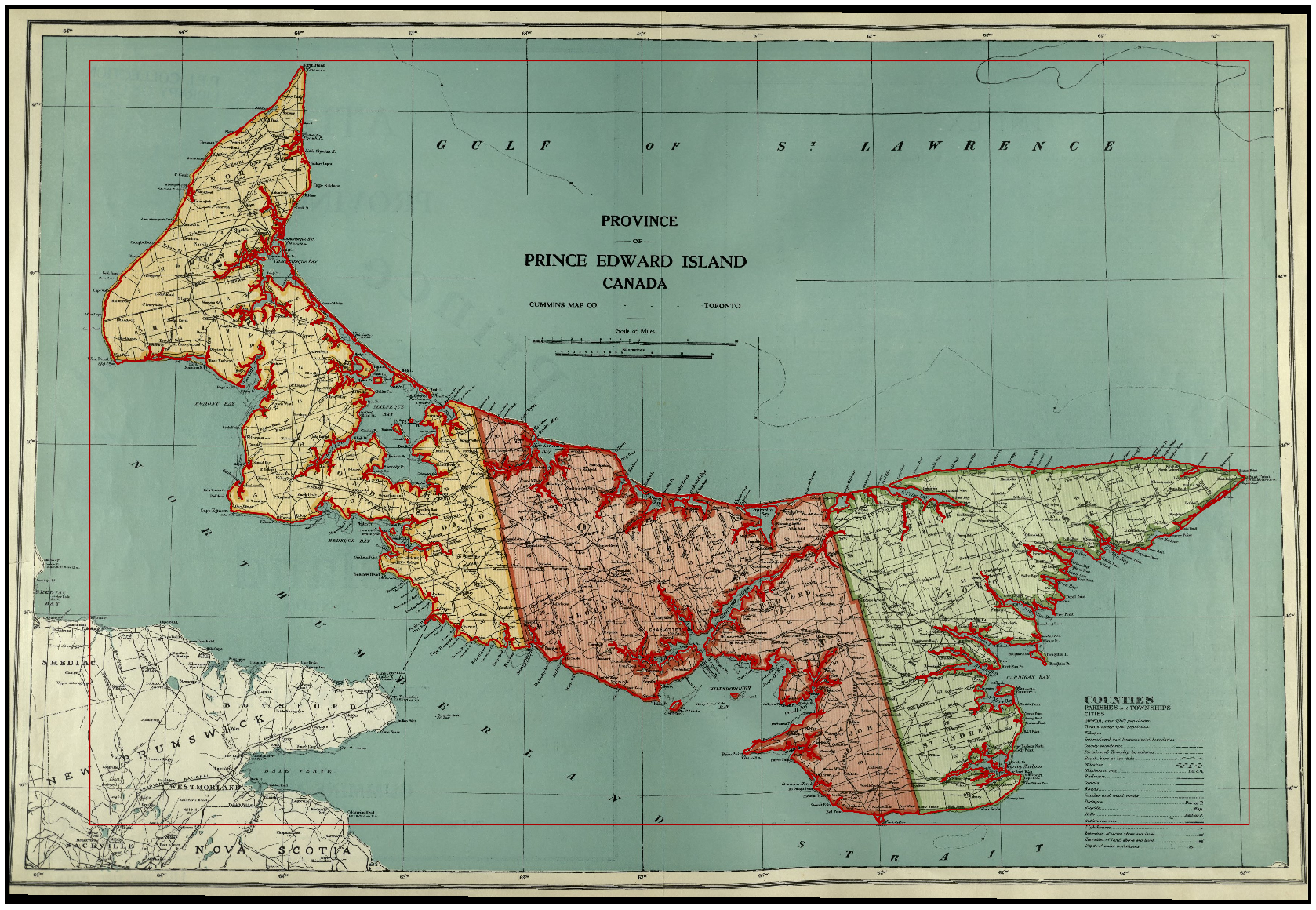
Figure 1: Click to see full size image.
We are now going to add a second historical map as a raster layer.
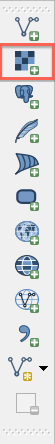
Figure 2
- under Layer on toolbar, choose Add Raster Layer (alternatively the same icon you see next to ‘Add Raster Layer’ can also be selected from tool bar)
- find the file you have downloaded titled ‘PEI_HollandMap1798’
- you will be prompted to define this layer’s coordinate system. In the Filter box search for ‘2291’ then in the box below select ‘NAD83(CSRS98) / Prince Edward Isl. Stereographic’
- If you are not prompted to define the layer’s coordinate system, you need to change a setting. Click Settings and then Options. Click CRS on the right hand menu and then choose ‘Prompt for CRS’ from the options below ‘When a new layer is created, or when a layer is loaded that has no CRS’. Click OK. Remove the Holland Map (right click on it and click Remove) and try adding it again. This time you should be prompted for a CRS and you can select the NAD83 option (see above).
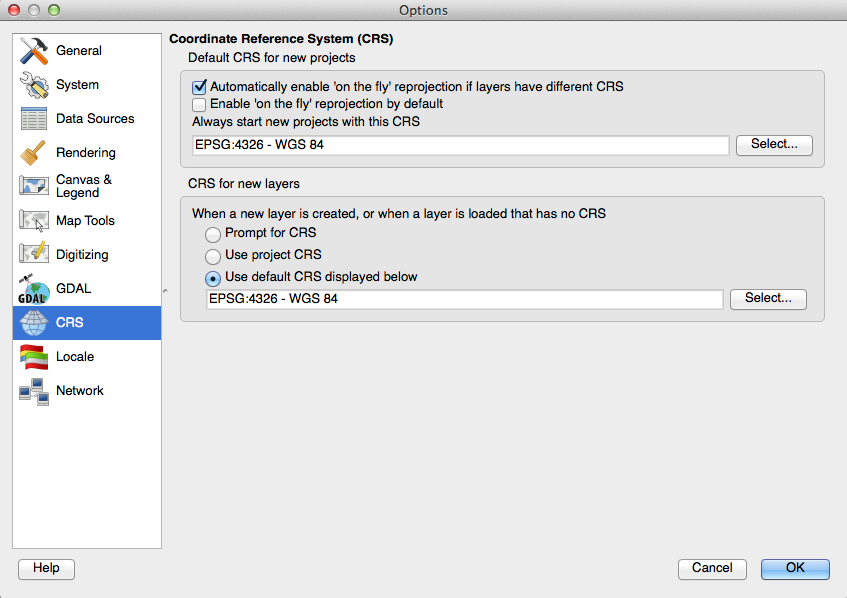
Figure 3
In previous steps you have selected and unselected layers in the Layers window by checking and unchecking the boxes next to them. These layers are organized in descending order of visibility – i.e. the layer at the top is the top layer in your viewer window (provided it is selected). You can drag the layers up and down in the Layer window to change the order in which they will be visible on your viewing window. The coastline_polygon raster layer is currently not visible because it is below the PEI_HollandMap1798 and PEI_Cummins1927 layers. In general it is best to keep vector layers above the raster layers.
Uncheck PEI_Cummins1927 so that the only layer you have remaining is PEI_HollandMap1798. Note that the map appears crooked on the screen; this is because it has already been georeferenced by the lesson writers to match the GIS vector layers. Learn more about georeferencing in Georeferencing in QGIS 2.0.
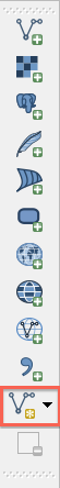
Figure 4
We will now create a point shapefile, which is a vector layer. Click Layer -> New -> New Shapefile Layer
- alternatively you can select the New Shapefile Layer icon on the top of the QGIS toolbar window
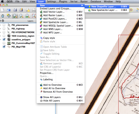
Figure 5
After selecting New Shapefile Layer, a window titled New Vector Layer appears
- In the Type category, Point is already selected for you. Click the Specify CRS button, and select NAD83(CSRS98) / Prince Edward Isl. Stereographic (EPSG: 2291), and then click OK (more information on understanding and selecting UTM zone).
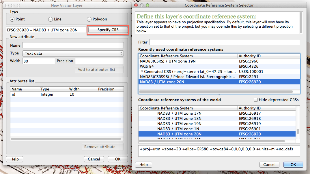
Figure 6: Click to see full size image.
Returning to the New Vector Layer window, we are going to make some attributes. To create the first attribute:
- under New attribute, in the field beside Name, type in ‘Settlement_Name’ (note that when working in databases you cannot use empty spaces in names so the convention is to use underscores in their place)
- click Add to attributes list
Now we are going to create a second attribute:
- under New attribute, in the field beside Name, type in ‘Year’
- this time, we are going to change the Type to Whole Number
- click Add to attribute list
For the third attribute:
- under New attribute, in the field beside Name, type in “End_Year” (GIS is not always optimal for dealing with change over time, so in some cases it is important to have a field to identify approximately when something ceased to exist)
- change the Type again to Whole Number
- click Add to attribute list
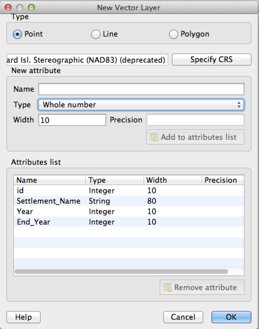
Figure 7
- When you complete these three steps, finish creating this shapefile by clicking OK on the bottom right of the New Vector Layer window. A pops up – name it ‘settlements’ and save it with your other GIS files.
Note that a layer called ‘settlements’ now appears in your Layers window. Relocate it above the raster layers.
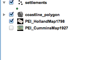
Figure 8
Uncheck all layers except settlements. You will notice that your viewing
window is now blank as we have not created any data. We will now create
new data from both the PEI_HollandMap 1798 and the
PEI_CumminsMap1927 to show the increase in settlement between the late
18th and early 20th centuries.
- we will begin with the more recent, and thus usually more accurate, map. Reselect (i.e. check the boxes beside) coastline_polygon and PEI_CumminsMap1927
- in your viewing window, zoom in to Charlottetown (hint: Charlottetown is near the middle of the island on the south side, at the confluence of three rivers)
- select settlements layer in Layers window
- on the menu bar, select Toggle Editing
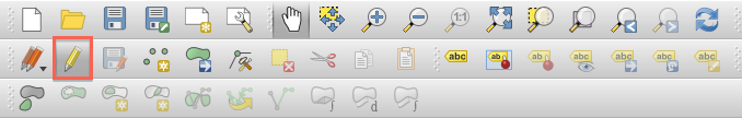
Figure 9
- After selecting Toggle Editing, editing buttons will become available to the right along the menu bar. Select the 3 dot feature button.

Figure 10
- Your cursor now appears as a crosshair – point the crosshair at Charlottetown (if you don’t happen to know PEI’s geography, you can cheat by adding on the PEI_placenames layer) keeping it within the modern day coastline, and click (digitization is always a compromise between accuracy and functionality; depending on the quality of the original map and the digitization, for most historical applications extreme accuracy is not necessary).
- An Attributes window will appear. Leave id field blank (at time of writing, QGIS appears to be making two id fields and this one is unnecessary). In Settlement field, type in ‘Charlottetown’. In the Year field type in 1764. Click OK
We will now repeat the steps we took with Charlottetown for Montague, Summerside, and Cavendish (again, you can find these locations by adding the PEI_placenames layers). Find Montague on the map, select the 3 dot feature button and click on Montague on the map. When the Attributes window appears, input Montague and 1732 in the appropriate fields. Repeat for Summerside (1876) and Cavendish (1790).
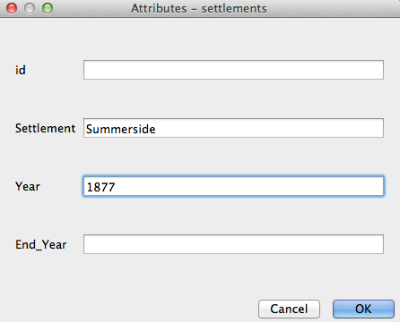
Figure 11
In the Layers window, unselect the PEI_CumminsMap1927 and select PEI_HollandMap1798. We are now going to identify two settlements (Princetown & Havre-St-Pierre) that no longer exist.
-
To locate Princetown, look for Richmond Bay and Cape Aylebsury (on the north coast to the west of Cavendish), here you will find Princetown (shaded-in) near the boundary between the yellow and the blue
-
If you look at the Wikipedia entry for the city you will notice that because of a shallow harbor, Princetown did not become a major settlement. It was renamed in 1947 and later downgraded to a hamlet. For this reason we will include 1947 as the end date for this settlement.
-
With the crosshair click on Princetown. In the Attribute table that appears, put Princetown in the Settlement field, put 1764 into the Year field, and put 1947 into the End_Year. Click OK
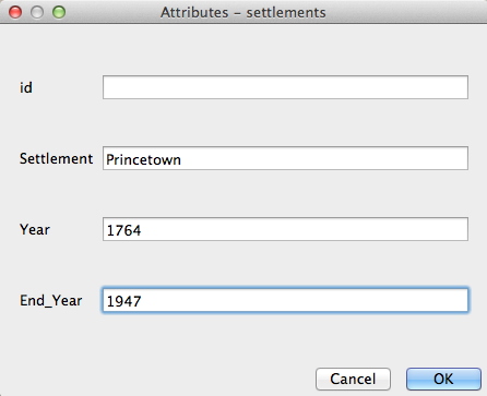
Figure 12
-
Click on Save Edits icon on the menu bar (it is between Toggle and Add Feature)
-
Double-click on settlements layer in the Layers window, choose Labels tab at the top of the ensuing window. Click on the box beside Display labels. In Field containing label select Year (if necessary), change font size to 18.0, change Placement to Above Left, and then click OK
On the northern coast of Lot 39 between Britain’s Pond and St. Peters Bay, we will now put a dot for the location of a long lost village called Havre-St-Pierre.
-
Havre-St-Pierre was the island’s first Acadian settlement but has been uninhabited since the Acadian deportation of 1758.
-
With the crosshair click on Havre-St. Pierre. In the Attribute table that appears, put Havre-St-Pierre in the Settlement field, put 1720 into the Year field, and put 1758 into the End_Year. Click OK
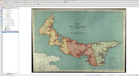
Figure 13
We will now now create another vector layer – this layer will be a line vector. Click Layer -> New -> New Shapefile Layer. The New Vector Layer window will appear (in the Type category at the top, select Line)
- Click the Specify CRS button, and select NAD83(CSRS98) / Prince Edward Isl. Stereographic (EPSG: 2291), and then click OK
- under New attribute, in the field beside Name, type in ‘Road_Name’
- click Add to attributes list
Create a second attribute
- under New attribute, in the field beside Name, type in Year
- change the Type to Whole Number
- click Add to attribute list
- To finish creating this shapefile, click OK on the bottom right of the New Vector Layer window. A ‘save’ screen pops up – name it ‘roads’ and save it with your other GIS files.
We are now going to trace the roads from the 1798 map so that we can compare them to the modern roads. Make that you have the PEI_Holland1798 and settlements layers checked in the Layers window. Select road layer in the layers window, select Toggle Editing on the top toolbar, and then select Add Feature

Figure 14
- First trace the road from Charlottetown to Princetown. Click on Charlottetown and then click repeatedly at points along the road to Princetown and you will see the line being created. Repeat until you arrive at Princetown, then right-click. In the resulting Attributes – road window, in the Name field enter “to Princetown” and in the Year field enter 1798. Click OK
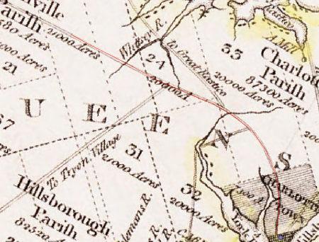
Figure 15
- repeat this step for 3 to 4 more roads found on the PEI_HollandMap1798.
- click Save Edits and then click Toggle Editing to turn it off
Deselect the PEI_HollandMap1798 in the Layers window and select the PEI_highway map. Compare the roads represented in the PEI_highway map (the red dotted lines) to the roads you have just traced.
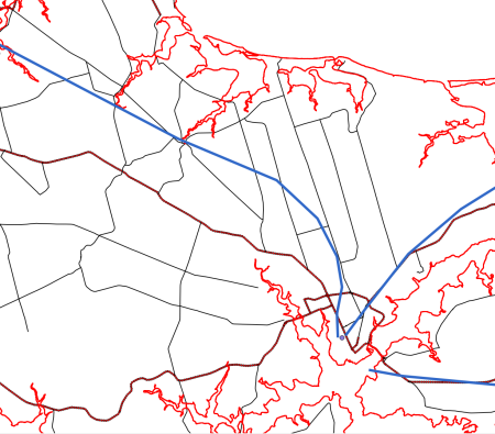
Figure 16
- We can see that some of these roads correspond closely to modern roads, while others do not at all correspond. It would take further historical research to determine whether this is simply because the Holland map did not sufficiently survey roads at the time, or if roads have changed considerably since then.
Now create a third type of vector layer: a polygon vector. Click Layer -> New -> New Shapefile Layer. The New Vector Layer window will appear – in the Type category at the top, select Polygon
- Click the Specify CRS button, and select NAD83(CSRS98) / Prince Edward Isl. Stereographic (EPSG: 2291), and then click OK
- under New attribute, in the field beside Name, type in ‘lot_name’ in the field beside Year
- click Add to attributes list
Create a second attribute
- under New attribute, in the field beside Name, type in Year
- change the Type to Whole Number
- click Add to attribute list
Figure 17
Start by creating a polygon for lot 66, which is the only rectangular lot on the island
- Click on Toggle Editing on top tool bar, and then click on Add Feature
- click on all four corners of lot 66 and you will see a polygon created
- right-click on the final corner and an Attributes window will appear. Add 66 to lot_names field and add 1764 (the year these lots were surveyed) to the Year field
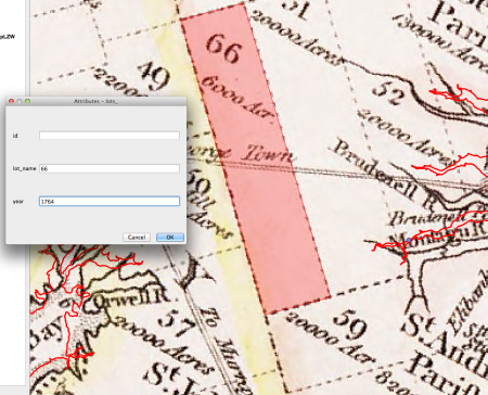
Figure 18
We are now going to trace lot 38, which is just west of Havre-St-Pierre. Make sure that there is a check mark in the box beside PEI_HollandMap1798 layer in the Layers window
Click on Toggle Editing on top tool bar, and then click on Add Feature
Trace the outline of Lot 38, which is more difficult because of the coastline, as accurately as possible. In order to show you the Snap feature, we want you to trace along the modern coastline (snapping is an automatic editing operation that adjusts the feature you have drawn to coincide or lineup exactly with the coordinates and shape of another nearby feature)
- select Settings-> Snapping Options
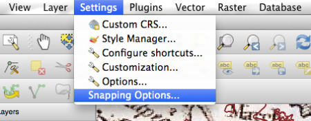
Figure 19
- a Snapping options window will open: click on the box beside coastal_polygon, for the Mode category select “to vertex and segment”, for Tolerance select 10.0, and for Units select ‘pixels’. Click OK
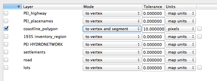
Figure 20
Make sure that the lots layer is selected in Layers window, and select Add Feature from the tool bar
- with your cursor click on the two bottom corners of your polygon just as you did with Lot 38. At the coastline you will notice that you have a collection of lines to trace around Savage Harbour. This is where the Snapping features becomes helpful. As you work to trace along the modern coastline it will significantly improve your accuracy by snapping your clicks directly on top of the existing line. The more clicks you make the more accurate it will be, but keep in mind that for many HGIS purposes obtaining extreme accuracy sometimes produces diminishing returns.
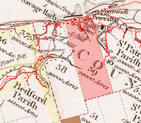
Figure 21
When you finish tracing and creating the polygon, select and deselect the various layers you have created, comparing and seeing what relationships you can deduce.
In Google Earth there were limitations on the types of features, attributes, and data provided by Google, and Google Earth did much of the work for you. That is fine when you are learning or want to quickly create maps. The advantage of using QGIS software to create new vector layers is that you have a great deal of freedom and control over the types of data you can use and the features and attributes that you can create. This in turn means that you can create custom maps far beyond what can be achieved in Google Earth or Google Maps Engine Lite. You have seen this firsthand with the points, lines, and polygons vector layers you learned how to create in this lesson. If you found data on, for example, public health records in the 18th century, you could create a new layer to work with what you already created showing the distribution of typhoid outbreaks and see if there are correlations with major roads and settlements. Moreover, GIS software allows you to not only spatially represent and present data in much more sophisticated ways, but to analyze and create new data in ways that aren’t possible otherwise.
You have learned how to create vector layers. Make sure you save your work!
This lesson is part of the Geospatial Historian.