
Contents
- Introduction
- Setup and Dataset
- Understanding Neural Networks
- Creating Your Own Model
- Conclusion
- References
- Endnotes
Introduction
In the last few years, machine learning has transformed computer vision and impacted a myriad of industries and disciplines. These innovations have enabled scholars to conduct large-scale explorations of cultural datasets previously requiring manual interpretation, but also bring their own set of challenges. Bias is rampant, and many machine learning techniques disproportionately damage women and communities of color. Humanities scholars with expertise in issues of identity and power can serve as important bulwarks against growing digital inequality. Yet, the high level of statistics and computer science knowledge required to comprehend machine learning algorithms has resulted in critical analysis often failing to look inside the ‘black box’.
This lesson provides a beginner-friendly introduction to convolutional neural networks, which along with transformers, are frequently-used machine learning models for image classification. Neural networks develop their own idiosyncratic ways of seeing and often fail to separate features in the ways we might expect. Understanding how these networks operate provides us with a way to explore their limitations when programmed to identify images they have not been trained to recognize.
In this tutorial, we will train a convolutional neural network to classify paintings. As historians, we can use these models to analyze which topics recur most often over time, or automate the creation of metadata for a database. In contrast to other resources that focus on developing the most accurate model, the goal of this lesson is more modest. It is aimed at those wanting to gain an understanding of the basic terminology and makeup of neural networks so that they can expand their knowledge later, rather than those seeking to create production-level models from the outset.
Audience and Requirements
Neural networks are a fascinating topic, and I have done my best to simplify my explaination of them. Although this removes some nuance, it also allows us to more easily gain an understanding of the general concept and how neural networks operate. Nonetheless, because of the issue’s complexity, this tutorial provides more background information than other tutorials focused on advanced coding.
We will be using Google’s Teachable Machine to train our model — don’t worry if you don’t know what “training” a model is right now. Teachable Machine contains a drag and drop interface that permits even those without coding experience to train a model. While the default model we create in Teachable Machine will be biased towards our training data, it will suffice for pedagogical purposes and make apparent machine learning’s limitations.
The latter half of the tutorial will take the neural network we train in Teachable Machine and embed it into a live website. To follow along with this section, you will need to have some familiarity with coding JavaScript. We will be using the ml5.js JavaScript library built on top of Tensorflow.js. This library takes its inspiration from Processing and p5.js created by The Processing Foundation whose goal is “to promote software literacy within the visual arts, and visual literacy within technology-related fields — and to make these fields accessible to diverse communities.”[1^] For those needing a JavaScript refresher, FreeCodeCamp has excellent and free interactive tutorials. I also recommend Jon Duckett’s book JavaScript and jQuery: Interactive Front End Development1. If neither of these resources appeal to you, there are hundreds of additional tutorials and videos you can access online through a quick search.
Along with JavaScript, you should have some familiarity with your browser’s developer tools and know how to use load up the JavaScript console. If you need help, there are instructions for Chrome, Firefox, Edge, and Safari available. Many browsers limit access to local files through JavaScript for security reasons. Consequently, you will be likely to need to launch a live server on your machine. I recommend that you either use an extension for your code editor, such as Live Server for Visual Studio Code, or run a server through Python.
Hopefully, the choice of the tools in this tutorial will allow you to focus on the broader concepts surrounding neural networks without worrying as much about coding. It’s worth mentioning, however, that Python and R are vastly more popular at the production level, and much of the cutting-edge work in machine learning relies on these two languages rather than the toolset shown in this tutorial. If you are interested in expanding your knowledge of neural networks, see Programming Historian’s excellent articles on Computer Vision for the Humanities and Interrogating a National Narrative with Recurrent Neural Networks.
Setup and Dataset
To begin, create a new folder called projects. This folder will hold all relevant files and images. To train the neural network in Google’s Teachable Machine, you will need a collection of labeled images as most neural networks are geared towards what is known as ‘supervised learning’.
Machine learning can be divided into two forms: supervised and unsupervised learning. Supervised learning involves data that is already labeled. Unsupervised learning, on the other hand, involves identifying patterns and grouping data that is alike together. You may have seen the use of some unsupervised machine learning algorithms such as K-Means Clustering and Latent Dirichlet Allocation in digital humanities research.
For this tutorial, we will download a dataset of paintings from ArtUK, which provides access to works that meet the UK’s requirements for “public ownership.” Approximately, 80% of the UK’s publicly owned art is not on display. ArtUK combats this by providing the general public access to these materials.
The ArtUK website allows you to view artworks by topic, and we will use these topics to train our image classifier. You can download a .zip file containing the images here. Save the .zip file in your projects folder and unzip it. Inside, you will find a folder called “dataset” with two additional folders: training and testing. Once you have downloaded all the files, go ahead and launch a live server on the projects folder. In most cases, you can view the server using the localhost address of “http://127.0.0.1”.
Understanding Neural Networks
How exactly do artificial neurons work? Rather than diving directly into training them, it is helpful to first gain a broader understanding of their infrastructure.
Let’s say we are interested in a simple task, such as determining if an image is a picture of a square or triangle. If you have done any kind of coding, you will know that most programs solve this by processing a sequence of steps. Loops and statements (such as for, while and if) allow our program to have branches that simulate logical thinking. In the case of determining whether an image contains a shape, we could code our program to count the number of sides and display “square” if it finds four, or “triangle” if it finds three. Distinguishing between geometric objects may seem like a relatively simple task, but it requires a programmer to not only define a shape’s characteristics but also implement logic that discerns those characteristics. This becomes increasingly difficult as we run into scenarios where distinctions between images are more complex. For instance, look at the following images:

Figure 1. A picture of a cat

Figure 2. A picture of a dog
As humans, we can easily determine which one is a dog and which one is a cat. However, outlining the exact differences proves challenging. It turns out that humans are usually a lot better at handling the nuances of vision than computers. What if we could get a computer to process images the way our brains do? This question and insight forms the basis of artificial neurons.
As the name implies, artificial neurons take their inspiration from neurons in the brain. The following is a simplified diagram2 of how a biological and artificial neuron work:
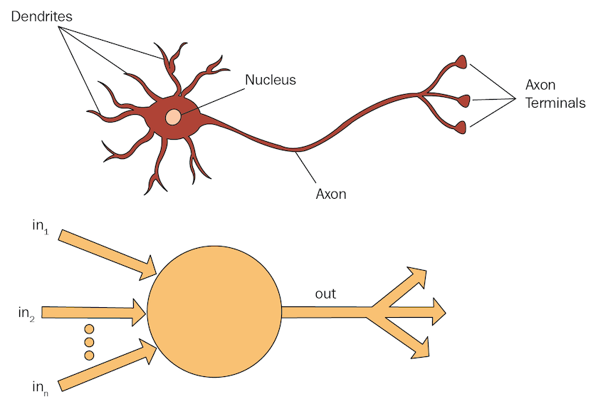
Figure 3. A diagram of a biological and an artificial neuron.
Biological neurons have dendrites, which are branch-like appendages that receive electrical inputs from other neurons and send those to the cell body. If stimulated enough, the cell body will send signals down the axon to the axon terminals which will then output them to other neurons.
In what ways does an artificial neuron mimic a biological one? In 1943, Warren MuCulloch and Walter Pitts laid the foundation for creating artificial neurons in their paper “A Logical Calculus of Ideas Immanent in Nervous Activity.”3 In contrast to biological neurons that receive their electricity from other neurons, they posited that an artificial neuron receives an arbitrary number of numerical values. It then outputs their sum to another neuron. This, however, presents a problem: if the neuron automatically outputs these sums, all neurons would fire simultaneously rather than when sufficiently stimulated. To counter this, artificial neurons determine if the sum of the inputs they receive exceed a particular threshold before outputting the results. Think of it as a cup that can hold a certain amount of liquid before it starts overflowing. Likewise, a neuron may take in electricity but only “fire” when it reaches a critical mass. The exact way that this threshold outputs to other neurons is determined through activation functions, which we will look at in more depth in the next section.
It should be noted that biological neurons are vastly more complex entities than artificial neurons. Andrew Glassner sums up the gulf between the two in Deep Learning a Visual Approach by noting:
The “neurons” we use in machine learning are inspired by real neurons in the same way that a stick figure drawing is inspired by a human body. There’s a resemblance, but only in the most general sense. Almost all of the details are lost along the way, and we’re left with something that’s more of a reminder of the original, rather than even a simplified copy.4
What is important to understand is not the exact relationship between artificial and biological neurons, but the spatial language and metaphors used in the literature which can make it much easier to figure out what exactly is going on in a basic neural network.
A Basic Neural Network
A neural network is simply a web of interconnected artificial neurons. Those we will examine here are ‘feed-forward’, which means that data only passes through them in one direction. These are particularly popular for completing classification tasks. In contrast, recurrent neural networks have loops where data from one part of the neural network is passed back to another. Although they are usually drawn from left to right, it is easier to think of a neural network as a series of steps where each neuron does some sort of calculation. They almost always consist of an input layer, a series of hidden layers, and an output layer.
As the name implies, the input layer holds the inputs for the data to be analyzed. Regardless of the data’s original form, it must first be converted into a numerical representation to go through the network. Let’s consider how neurons convert digital images to numbers. Digital images are made up of a series of pixels. We can represent these images numerically as multi-dimensional arrays with dimensions representing height, width, and the number of channels. The channels correspond to the color depth for each pixel. For instance, the color depth for a grayscale image will have a single value representing the intensity of light, while a color image will have a series of values for red, green, and blue.
From the input layer, the neural network usually passes data into a series of “hidden layers.” Hidden layers are those after the input layer and before the output layer. Depending on the type of network, the number of hidden layers and their function will vary. Any network with more than one hidden layer is referred to as a “deep neural network.”
In most hidden layers, the neural network takes the values from previous layers, does a mathematical calculation on them (usually summation), and multiplies the sum by a particular ‘weight’ before sending it to the neurons in the next layer. Each neuron then takes its input and turns it into a single output — normally by adding up the values.
How do the neurons in hidden layers help solve mathematical problems and classification tasks? Let’s go through a simple example. Let’s assume that we are interested in solving the following equation: x+y=7.5. In this scenario, we know that the output should be 7.5, but we do not know the inputs. We can begin by simply guessing numbers such as 3 and 2. Putting them into our equation gives us an answer of 5. However, we know that we need to get an answer of 7.5 so one of the things that we can do is multiply the inputs by a number. We can start by multiplying our original guesses by 2. The amount that we multiply each number is known as a weight: (3x2)+(2x2)=10. Now we have overshot our output, so we need to adjust the weights down. A neural network uses the “error” value to adjust the weights of our network accordingly, in a process called “back propagation.” Let’s try 1.5: (3x1.5)+(2x1.5)=7.5. We now have the correct result despite not knowing the original inputs and simply choosing two random values. This is exactly how a neural network works!
One thing to note is that the output of a neuron to the next layer is rarely the value originally calculated. Instead, it is sent to an activation function to prevent network collapse. Recall from earlier that an activation function in a biological neuron has a threshold that stops all neurons from firing at the same time. You can think of network collapse as removing any redundancy in neurons. For instance, if a neuron adds two different input values then outputs them to another neuron which, in turn, adds up the first neuron’s output, we can reduce the number of neurons by programming the first to perform the whole calculation. While this may seem more efficient, it diminishes our network’s flexibility.
The activation function in an artificial neuron stops network collapse by introducing non-linearity. There are numerous types of activation functions. The simplest non-linear functions are “step functions.” In these functions, a certain threshold (sometimes a group of thresholds) is chosen and the values to the left of the threshold output a single value, while the values to the right of the threshold output several values. The most popular activation functions are variations of rectified linear unit (ReLU). In its simplest form, a ReLU activation function outputs 0 for values that are less than zero, and the input value itself if it’s higher than zero.
Activation functions are particularly important in the final layer as they constrain the output to within a certain range. If you are familiar with logistic regression, you may be familiar with the sigmoid function which is used in binary classification. We can use this same function as an activation function for a neural network to constrain our values set to 0 or 1. However, because we normally have more than two categories, the ArgMax and SoftMax functions are more common. The former outputs the category with the maximum probability to 1 and the remainder to zero. The latter provides values for each category between 0 and 1 with the highest value indicating the most likely classification and the lowest value indicating the least likely classification.
Convolutional Neural Networks
Hopefully, you now have a good understanding of how a basic neural network works. Convolutional neural networks draw on this same foundation. These networks are particularly good at detecting image features and get their name from their “convolutional layers.”
Think about what makes up an image. If you have ever taken a drawing class, you may have learned to divide a sketch into simple shapes, such as circles and squares. Later, you took these shapes and drew more complex images on top of them. A convolutional neural network essentially does the same thing. As we stack convolution layers on top of one another, each learns to identify different parts of a growingly complex shape. The first layer detects basic features such as corners and edges. The middle layers detect shapes and segment them into object parts. The last layers will be able to recognize the objects themselves, before sending them to the output layer for classification. For more information about how the layers of a convolution network work, I recommend Erik Reppel’s excellent blog post Visualizing parts of Convolutional Neural Networks using Keras and Cats.5
What exactly is a convolution though? At its most basic, a convolution is a mathematical function resulting in two sets of information becoming converged. If you have used filters, such as blurs, in common image editing applications, you have used convolutions. Convolutions for images work by taking a filter (also known as a kernel) consisting of a grid of numbers; usually 3x3 or 5x5, and moving it over each pixel in the image. As the filter moves, the values in each overlapping pixel are multiplied by the values in the filter. Finally, the values for all the numbers in the grid are added together to create a single output.
Because the neural network takes the values from each grid and adds them together, the values given to the next layer are smaller than the original image. This new array of numbers is referred to as a “feature map” and makes training the neural network less computationally intensive. An activation function, such as ReLU, is also commonly used to transform all negative values to zero.
Finally, a “pooling layer” is utilized. A pooling layer works similarly to a convolutional layer in that it takes a grid; usually 2x2, and passes it over each value in the feature map. In contrast with the convolution layer, however, the pooling layer simply takes the maximum or average value (depending on which convolutional neural network you are using) of the numbers in the grid. This creates a smaller feature map. Together, convolutions and pooling allow neural networks to perform image classification even if the spatial arrangement of the pixels is different, and without having to do as many calculations.
Transfer Learning and Convolutional Neural Networks
Now, we are going to begin using Google’s Teachable Machine to train our model. Teachable Machine provides a simple interface we can use without initially having to worry about code. When you load it, you will find that you have the option to train three different types of models. For this tutorial, we will be creating what Teachable Machine calls a “Standard image model.”
Training an image classifier from scratch can be difficult. We would need to provide numerous images along with their corresponding labels. Instead, Teachable Machine relies on transfer learning.
Transfer learning expands on a model that has already been trained on a separate group of images. Teachable Machine relies on MobileNet as the basis for its transfer learning. MobileNet is a lightweight neural network designed to run on small devices with low-latency. Its training times are relatively quick, and we can start with fewer images. Of course, MobileNet was not trained on the images that we are interested in, so how exactly can we use it? This is where transfer learning kicks in.
You can think of transfer learning as a process of modifying the final layer of a preexisting model to discern our images’ “features.” At first, these features are mapped to the categories that MobileNet was trained on, but through transfer learning, we can overwrite this mapping to reflect our own categories. Thus, we can rely on the earlier layers to do most of the heavy lifting —detecting basic features and shapes— while still having the benefit of using the final layers to recognize specific objects and perform classification.
Creating Your Own Model
On the Teachable Machine home page, go ahead and click the “Get Started” button. Then, click “Image Project” and select “Standard image model.”
Now, we can begin uploading image samples for each class. You will find that you can either “Upload” images or use your webcam to create new ones. We will be uploading all the images for each of our categories to the training folder.
Under “Class 1”, click “Choose images from your files, or drag & drop here.” Select the “aircraft” folder from inside the dataset “training” folder and drag it into the Teachable Machine window. Click the pencil icon next to “Class 1” and change the name to “aircraft”.
Repeat this process for the other folders in the dataset. After the second time, you will need to click “+ Add a class” for each new folder.
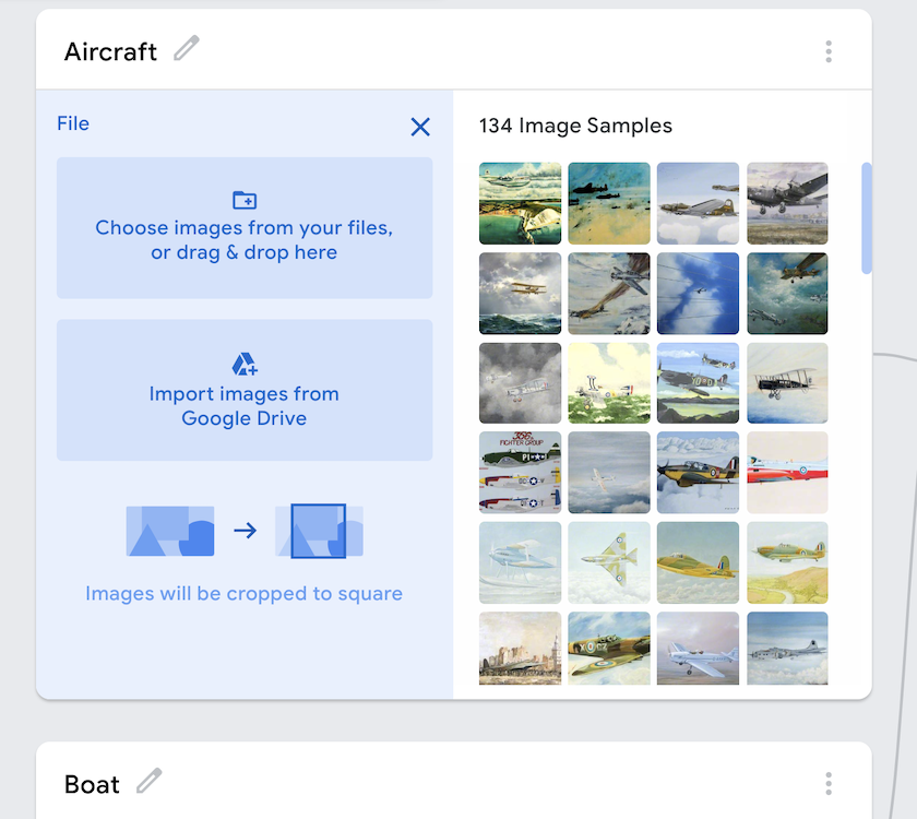
Figure 4. Adding classes to Google Teachable Machine.
Once you have finished uploading the images, you can adjust various parameters for how the model should be trained by clicking on “Advanced” under Training. Here you will see options for epochs, batch size, and learning rate.
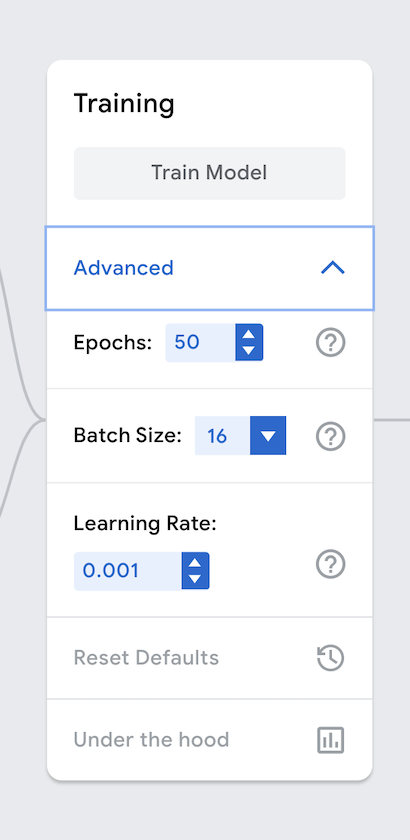
Figure 5. Advanced settings in Google Teachable Machine.
An epoch refers to the number of times that each image is fed through the neural network during training. Because each image is fed through multiple times, we don’t actually need a large number of sample images. You may be wondering why we don’t just set the epoch ridiculously high so that our model works through the dataset a greater number of times. The chief reason is “overfitting.”
Overfitting is when our neural network gets really proficient at working with our training set but fails on new data. This is a result of the bias-variance tradeoff. If a model has high bias, it performs well on our training data set but not as well on a new one. In contrast, if it has high variance, it may not work as well on our training data but could have more flexibility when it comes to new data. How to determine the exact relationship between variance and bias is a complex topic. One common method is to save a bit of the original data by splitting it into a “testing” set. Rather than using this data to build the original model, the testing set is used to provide statistical summaries of how well the model will work on new data. Teachable Machine does this ‘under the hood’, but when you build more elaborate models, you will need to determine how much of the original data should be preserved yourself.
Batch size refers to the number of images used for training per iteration. If you have 80 images and a batch size of 16, this means that it will take 5 iterations to make up one epoch. A key advantage to using a smaller batch size is that it is much more efficient on memory. Because we are updating the model after each batch, the network tends to be trained faster. Nonethless, batch sizes make an impact on the generalization and convergence on our model, so we need to be careful with this setting.
The learning rate refers to how much we should change our model based on the estimated error. This impacts how well your neural network performs.
We will stick with the default settings for now. Click on the “Train” button to begin training your model.
A bar will display the progress. Be sure not to close your browser or switch tabs during this time. The pop-up displayed below will remind you of this.

Figure 6. Pop-up Showing Not to Switch Tabs
After training is complete, you will want to test your model. There are various measures we can use to determine how well a model works. If you click on “Under the hood” in the Advanced settings, the Loss and Accuracy per Epoch is displayed. The closer the loss is to 0 and the accuracy is to 1, the better our model is at understanding our images.
One of the benefits of Teachable Machine is that we can immediately begin testing our model. The default input for new images is to use your webcam so we will switch it to file. Go ahead and upload one of the images in the testing folder and see the results. Normally we would want to test our model with many images at once, but Teachable Machine only lets us test one image at a time. In the testing folder, there are ten images for testing the classification. Go ahead and compare how you would classify them yourself with the output Teachable Machine provided.
Export the Model
Let’s export and download our model to see how we can reuse it in new circumstances. Click the “Export Model” button, and you will see three options: Tensorflow.js, Tensorflow, and Tensorflow Light. Tensorflow is a library developed by Google focused on machine learning and artificial intelligence. We will choose Tensorflow.js, which is simply a JavaScript implementation of the library. Ml5.js and p5.js, which we will use to later embed our model on our website, rely on Tensorflow.js at a lower level.
Once you have selected Tensorflow.js, you will be given a .zip file containing three files:
model.jsoncontaining data about the different layers for the neural network itselfweights.bincontaining information about the weights for each of the neuronsmetadata.jsoncontaining information about which Tensorflow version is being used for the network along with the class labels
Unzip this folder, and place the files inside of your projects folder:
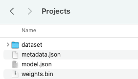
Figure 7. Projects Folder with Tensorflow.js Files
Import the Model with ml5.js
Teachable Machine is a great resource for familiarizing yourself with how neural networks —and machine learning more broadly— work. However, it is limited in what it can do. For instance, maybe we would like to create some sort of graph that displays information about the classification. Or, maybe we want to allow others to use our model for classification. For that, we will need to import our model to a system that allows more flexibility. Although there are many possible tools to choose from, for this tutorial we will be using ml5.js and p5.js.
Ml5.js is a JavaScript library built on top of Tensorflow.js. As mentioned earlier, machine learning libraries often require users to have significant background knowledge of programming and/or statistics. For most neural network libraries, you must specify properties for each layer of the neural network such as its inputs, outputs, and activation functions. Ml5.js takes care of this for you, making it easier for beginners to start.
To begin, let’s go ahead and create some files in our projects folder. Inside the folder, we will create an index.html page that will call the rest of our JavaScript libraries. This allows us to examine the model’s output without having to look directly at the browser’s developer console — although we will do that as well. We also need to create a file called sketch.js in the same directory as index.html.
In the discussion below, we will add the contents of this file step by step. If you get lost at any point, you can download the full code here.
Finally, we will take an image from the testing folder and place it in our project’s root folder to assure our code is working. You can use any image you like, but I am going to use the first one for this example. Your projects folder should now look like this:
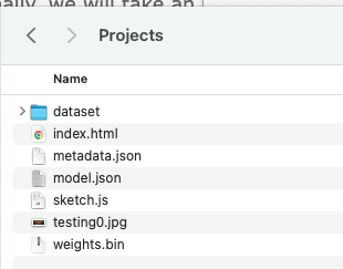
Figure 8. Projects Folder with ‘script.js’, ‘index.html’, and test image
We will base the code for our index.html file on the official ml5.js boilerplate template. This template links to the latest ml5.js and p5.js libraries. While ml5.js does not require p5.js, most examples use both because the combination allows us to quickly code an interface for interacting with the model. We will have most of the code for our neural network in a separate JavaScript file named sketch.js, and our boilerplate template will link to that script.
<!DOCTYPE html>
<html lang="en">
  <head>
    <title>Getting Started with ml5.js</title>
    <meta name="viewport" content="width=device-width, initial-scale=1.0">
    <!-- p5 -->
    <script src="https://cdnjs.cloudflare.com/ajax/libs/p5.js/1.0.0/p5.min.js"></script>
    <!-- ml5 -->
    <script src="https://unpkg.com/ml5@latest/dist/ml5.min.js"></script>
    <script src="sketch.js"></script>
  </head>
  <body>
  </body>
</html>
Outside of this template, we do not have any additional code in our index.html file. Instead, we have a link to sketch.js. Note that many p5.js and ml5.js conventions draw on artistic terminology, and that is where we will do the majority of our coding. Switch your editor to sketch.js.
We will make sure that everything is working properly by printing the current version of ml5.js to the console. In sketch.js, copy or type the following:
// Output the current version of ml5 to the console
console.log('ml5 version:', ml5.version);
You should have already started a live server during the setup stage. If not, you should launch it now on the projects folder. Load up index.html in your web browser —remember that index.html is just a boiler plate template linking to sketch.js— and check the developer console for the output. As long as the output for the current version displays, you shouldn’t encounter any problems.
Because we are using p5.js, it is worth taking a few minutes to examine some of its peculiarities. P5.js is an interpretation of Processing in JavaScript. Both p5.js and Processing cater to digital artists, especially those interested in creating generative art. You will find that drawing on artistic terminology is a common convention amongst p5.js and ml5.js programmers. This is why we named our JavaScript file sketch.js.
The two key functions in p5.js that draw on this tradition are the setup() and draw() functions. The setup() function is automatically executed when the program is run. We will use it to create a blank square canvas that is 500x500 pixels using the createCanvas() function. We will also move our code that outputs the current version of ml5.js to the console.
function setup() {
    // Output the current version of ml5 to the console
    console.log('ml5 version:', ml5.version);
    // Create a blank square canvas that is 500px by 500px
    createCanvas(500,500);
}
By executing the command above you will have created the canvas but, because it is set to white, you may not be able to differentiate it from the rest of the page. To make it easier to see the boundaries of our canvas, we will use the background() function and pass it the hex value for black.
function setup() {
    // Output the current version of ml5 to the console
    console.log('ml5 version:', ml5.version);
    // Create a blank square canvas that is 500px by 500px
    createCanvas(500,500);
    // Set the background of the canvas to black based on the hex code
    background('#000000');
}
If you load index.html again, you will see that we now have a black canvas that is 500x500 pixels.
Next, we will load the actual model. In the past, this was commonly done using a callback function to deal with JavaScript’s asynchronous nature. If you are unfamiliar with JavaScript, this may be a source of confusion. Basically, JavaScript reads code from top to bottom, but it does not stop to complete any part of the code unless it must. This can lead to issues when performing tasks such as loading a model, because JavaScript may start calling the model before it has finished loading. Callback functions provide a way around this as they are not called in JavaScript until other code has already completed.
To deal with common errors in loading images, models and the complexity of callbacks, p5.js introduced a new preload() function. This is a powerful feature of p5.js that allows us to be sure that images and models are loaded before the setup() function is called.
We will place the call for loading our model in the preload() function and assign it to a global variable. Although the preload() function allows us to avoid callbacks in certain situations, we probably still want some feedback for when the model is successfully loaded. For this, we will create a new function called teachableMachineModelLoaded() that will output a message to the console. You only have to call the model.json file for this to work. Ml5.js will automatically look in the same folder for the file containing the weights and metadata.
// Variable to hold the machine learning model
let classifier;

 // Load model.json and set it to our variable. Make callback to teachableMachineModelLoaded function to output when loading is complete.
function preload() {
    classifier = ml5.imageClassifier('model.json', teachableMachineModelLoaded);
}

// Callback for assuring when model has completely loaded
function teachableMachineModelLoaded() {
  console.log('Teachable Machine Model Successfully Loaded!');
}
Now that we have loaded the model, we need to add our testing image. The first thing that we will do is load our image using the p5.js loadImage() function. The loadImage() function takes a path to the image as a parameter and returns a p5.Image object, which provides some additional functions to manipulate images compared with plain JavaScript. We can place this call in the preload() function. You can choose any of the test images or your own image to experiment with. Just place them in the same folder as the code. For the purposes of this tutorial, we are just going to load testing0.jpg, which is an image of an aircraft.
let classifier;
let testImage;

function preload() {
  classifier = ml5.imageClassifier('model.json', teachableMachineModelLoaded);
  // Load image from same folder. Note that you can change this to any image you want.
  testImage=loadImage("testing0.jpg");
  console.log("Successfully Loaded Test Image");
}
We can now use the p5.js image() function to draw the image to the screen. It takes three arguments. The first is the name of the variable containing the image. In this case, it is the testImage variable. The next two are x and y coordinates for where to place the image. We are going to put it in the center of our canvas. An easy way to do this is through the “height” and “width” variables that contain the canvas dimensions. P5.js makes these available to us automatically, and we can divide by two to center the image.
We will issue this call inside of the draw() function, which is called immediately after setup() and is where we will place the majority of our code.
function draw() {
    // Place image in center by dividing canvas width and height by two.
    image(testImage, width/2, height/2);
}
If you look at the image, you will find that it is not perfectly centered on the canvas. This is one of the peculiarities of working with p5.js. It places the image on the canvas using the top left corner as the anchor point. We can call the imageMode() function and pass it the “CENTER” argument to change how p5.js determines where to place images. This setting will stay in place until you decide to change it.
If you run the following, you will now see that we have our image in the center of the canvas.
function draw() {
    // Center image anchoring point to be center of image
    imageMode(CENTER);
    image(testImage, width/2, height/2);
}
The draw() function is unique to p5.js and loops based on the frame rate. This is again due to p5.js being originally geared towards artists. Constantly looping the material inside of draw() makes it easier to make animations. When you post the image onto the canvas, p5.js is actually continuously running the code and placing a new image on top of the old one. To stop this, we can call the noLoop() function.
function draw() {
    // Stop looping of code in draw
    noLoop();
    // Place anchor point of image in the center of the image
    imageMode(CENTER);
    // Output image to the center of the canvas
    image(testImage, width/2, height/2);
}
We are now ready to evaluate our model. We will call the classify() function from our classifier object. It requires a single argument containing the object that we are interested in classifying along with a callback. We will use getResults() as our callback function. ml5.js will automatically send two arguments to the function containing information about errors and/or results. We will output these results to the console:
function draw() {
  noLoop();
  imageMode(CENTER);
  image(testImage, width/2, height/2);
  // Call classify function to get results. Use callback function called getResults to process the results
  classifier.classify(testImage, getResults);
}

function getResults(error, results) {
  // If there is an error in the classification, output to the console. Otherwise output the results to the console.
  if (error) {
    console.error(error);
  } else {
    console.log(results);
  }
}
If everything went well, you should see the results of the classification on the console as a JavaScript object. Let’s take a closer look at the output. Note that the exact numbers you get may vary. This is the output from the first image:
(5) [{...}, {...}, {...}, {...}]
0: {label: 'Aircraft', confidence: 0.6536924242973328}
1: {label: 'Boat', confidence: 0.3462243676185608}
2: {label: 'House', confidence: 0.000002019638486672193}
4: {label: 'Horse Racing', confidence: 1.42969639682633e-7}
length: 5
[[Prototype]]: Array(0)
If you look inside the JavaScript object (in most browsers, this is done by clicking on the arrow symbol next to the object name), you will see the output for the testing0.jpg image list all the possible classes by probability and confidence. We see that results[0] contains the most likely result with the label listed in results[0].label. There is also a confidence score in results[0]. Confidence provides a percentage value which indicates how certain our model is of the first label.
We can output these values to our canvas using the text() function in our getResults() call, which takes as arguments our text and the x, y coordinates for where we want to place it. I will place the text just below the image itself. We will also need to call some functions that detail how we want our text to be displayed. Specifically, we will use fill() with a hex value for the color text, textSize() for the size, and textAlign() to use the center of our font as an anchor point. Finally, we will round the confidence to two decimal points using the toFixed() function.
function draw() {
  noLoop();
  imageMode(CENTER);
  image(testImage, width/2, height/2);
  classifier.classify(testImage, getResults);
}

function getResults(error, results) {
  if (error) {
    console.error(error);
  } else {
    // Set the color of the text to white
    fill('#FFFFFF');
    // Set the size of the text to 30
    textSize(30);
    // Set the anchor point of the text to the center
    textAlign(CENTER)
    // Place text on canvas below image with most likely classification and confidence score
    text("Confidence " + (results[0].confidence*100).toFixed(2) + "%", width/2, height/2+165)
    text("Most Likely " + results[0].label, width/2 , height/2+200);
    // Output most likely classification and confidence score to console
    console.log("Most likely " + results[0].label);
    console.log("Confidence " + (results[0].confidence*100).toFixed(2) + "%",);
    console.log(results);
  }
}
Run the code above to see a result of what the image represents along with a confidence score. If the code ran successfully, you should see the following result (although please note that your confidence score is likely to differ):

Figure 9. Example result.
Conclusion
This lesson has provided you with an introduction to how neural networks function, and explained how you can use them to perform image classification. I have purposefully kept the code and examples simple, but I encourage you to expand upon the code that you have used here. For instance, you could add loops that instruct a model to go through a folder of images and output the results into a CSV file which contains topics, or charts the themes of larger corpora. You could also investigate the limitations of the neural network to identify areas where it does not work. For example, what happens when you upload an abstract painting or something that isn’t a painting at all? Exploring these weak points can lead to inspiration not only for academic but also creative work.
One thing to keep in mind is that our model is biased towards our training data. In other words, while it may be helpful for categorizing the ArtUK images, it may not function as well when it comes to new data.
References
While Teachable Machine and ml5.js provide a good starting point, this simplicity comes with a loss of flexibility. As mentioned earlier, you will likely want to switch to Python or R to do production-level machine learning. I recommend the Programming Historian’s tutorials on Computer Vision for the Humanities and Interrogating a National Narrative with Recurrent Neural Networks. Both include links to further resources which will help you to expand your knowledge.
If you are interested in developing broader knowledge of ml5.js, or learning more about the concepts that underpin neural networks, I also recommend the following:
-
3Blue1Brown has some wonderful videos that delve into the math of neural networks. 3Blue1Brown, Neural Networks, https://www.3blue1brown.com/topics/neural-networks.
- Dan Shiffman provides a good overview of using ml5.js and p5.js for machine learning on his YouTube channel. The Coding Train, Beginner’s Guide to Machine Learning in JavaScript with ml5.js, YouTube video, 1:30, March 4 2022, https://youtu.be/26uABexmOX4.
-
He also has a series of videos on building a neural network from scratch that covers the mathematical foundations for machine learning. The Coding Train, 10.1: Introduction to Neural Networks - The Nature of Code, YouTube video, 7:31, 26 June, 2017, https://youtu.be/XJ7HLz9VYz0.
-
The official ml5.js reference provides a comprehensive overview of how to perform image classification alongside other machine learning tasks. Ml5.js, Reference, https://learn.ml5js.org/#/reference/index.
-
Tariq Rashid’s book Make Your Own Neural Network provides an excellent and clear introduction for those interested in developing knowledge of machine learning. Tariq Rashid. Make Your Own Neural Network. CreateSpace Independent Publishing Platform, 2016.
-
Tijmen Schep’s interactive documentary is an excellent introduction to the dangers of machine learning and AI. Tijmen Schep, How Normal Am I?, https://www.hownormalami.eu/.
- Jeremy Howard and Sylvain Gugger’s book Deep Learning for Coders with fastai and PyTorch: AI Applications Without a PhD provides a great introduction machine learning. Although it utilizes Python, the examples are straight-forward enough for most beginners to follow, and are relatively simple to recreate in other languages. Jeremy Howard and Sylvain Gugger. Deep Learning for Coders with fastai and PyTorch: AI Applications Without a PhD. O’Reilly Media, Inc., 2020.
-
They also have a free companion video series that covers much of the material in the book. freeCodeCamp.org, Practical Deep Learning for Coders - Full Course from fast.ai and Jeremy Howard, YouTube video series, 2020, https://youtu.be/0oyCUWLL_fU.
-
Grokking Deep Learning by Andrew Task is a wonderful book that provides a gentle introduction to some of the more advanced mathematical concepts in machine learning. Andrew Task. Grokking Deep Learning. Manning Publications, 2019.
- David Dao curates a list of current of some of the dangerous ways that AI has been utilized and perpetuates inequality. David Dao, Awful AI, https://github.com/daviddao/awful-ai.
Endnotes
-
Jon Duckett, JavaScript and jQuery: Interactive Front End Development, (Wiley, 2014). ↩
-
Karthikeyan NG, Arun Padmanabhan, Matt R. Cole, Mobile Artificial Intelligence Projects, (Packt Publishing. 2019). ↩
-
McCulloch, W.S., Pitts, W. A logical calculus of the ideas immanent in nervous activity. Bulletin of Mathematical Biophysics 5, 115–133 (1943). https://doi.org/10.1007/BF02478259 ↩
-
Andrew Glassner, Deep Learning a Visual Approach, (No Starch Press, 2021), 315. ↩
-
Erik Reppel, “Visualizing parts of Convolutional Neural Networks using Keras and Cats”, Hackernoon, Accessed December 23, 2022, https://hackernoon.com/visualizing-parts-of-convolutional-neural-networks-using-keras-and-cats-5cc01b214e59. ↩