Contents
- Lesson Goals
- Getting Started
- Open the Necessary GIS Layers
- Open the Georeferencer Tool
- Georeference!
Lesson Goals
In this lesson, you will learn how to georeference historical maps so that they may be added to a GIS as a raster layer. Georeferencing is required for anyone who wants to accurately digitize data found on a paper map, and since historians work mostly in the realm of paper, georeferencing is one of our most commonly used tools. The technique uses a series of control points to give a two-dimensional object like a paper map the real world coordinates it needs to align with the three-dimensional features of the earth in GIS software (in Intro to Google Maps and Google Earth we saw an ‘overlay’ which is a Google Earth shortcut version of georeferencing).
Georeferencing a historical map requires a knowledge of both the geography and the history of the place you are studying to ensure accuracy. The built and natural landscapes change over time, and it is important to confirm that the location of your control points — whether they be houses, intersections, or even towns — have remained constant. Entering control points in a GIS is easy, but behind the scenes, georeferencing uses complex transformation and compression processes. These are used to correct the distortions and inaccuracies found in many historical maps and stretch the maps so that they fit geographic coordinates. In cartography this is known as rubber-sheeting because it treats the map as if it were made of rubber and the control points as if they were tacks ‘pinning’ the historical document to a three dimensional surface like the globe.
Getting Started
Before proceeding with georeferencing in Quantum GIS, we need to activate the appropriate Plugins. On the toolbar go to Plugins -> Manage and Install Plugins
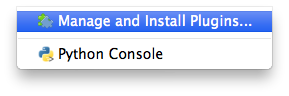
Figure 1
A window titled Plugin Manager will open. Scroll down to Georeference GDAL and check the box beside it, and click OK.
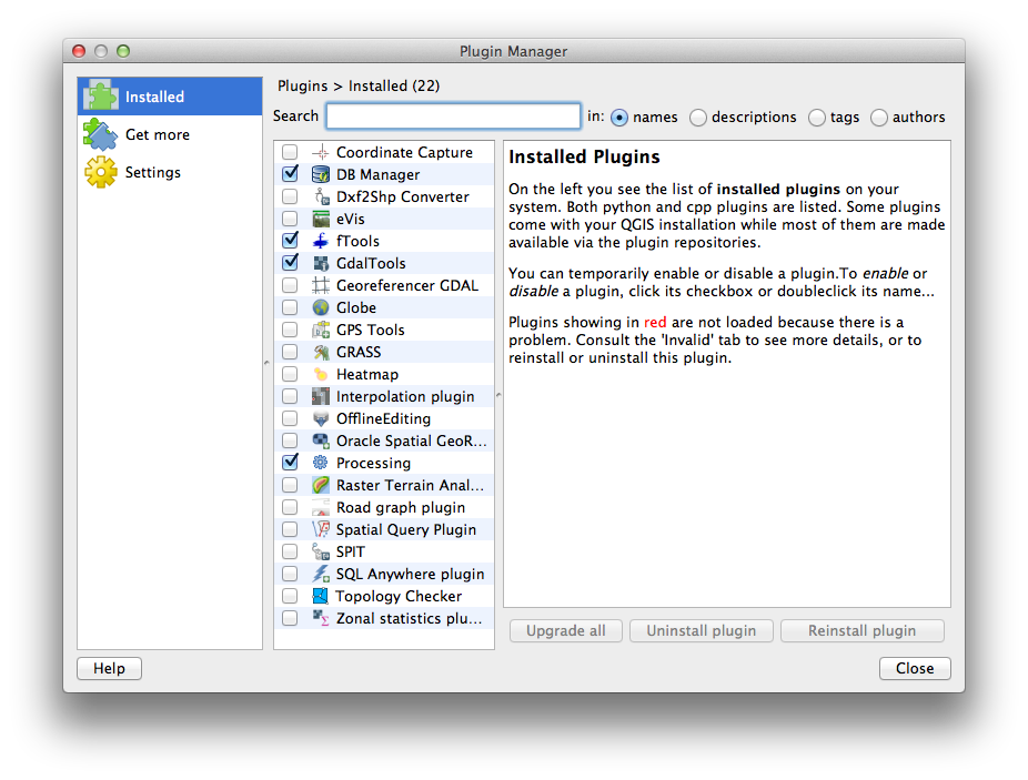
Figure 2
- At this point, you need to shut down and relaunch QGIS. For the purposes of this example, and to keep things as simple as possible, don’t reload your existing project but instead start a new project.
- Set up the Coordinate Reference System (CRS) correctly (see Installing QGIS 2.0 and adding Layers for a reminder)
- Save this new project (under File menu, select Save Project) and call it ‘georeferencing.’
- Add the ‘coastline_polygon’ layer (see Installing QGIS 2.0 and adding Layers for a reminder)
Open the Necessary GIS Layers
For the Prince Edward Island case study, we are going to use the township boundaries as control points because they were established in 1764 by Samuel Holland, they are identified on most maps of PEI, and they have changed very minimally since then.
Download lot_township_polygon:
This is the shapefile containing the modern vector layer we are going to use to georeference the historical map. Note that townships were not given names but rather a lot number in 1764, so they are usually referred to as ‘Lots’ in PEI. Hence the file name ‘lot_township_polygon’.
- Download the file:
- After downloading the file called ‘lot_township_polygon’, move it into a folder that you can find later and unzip the file. (Remember to keep the files together as they are all required to open this layer in your GIS)
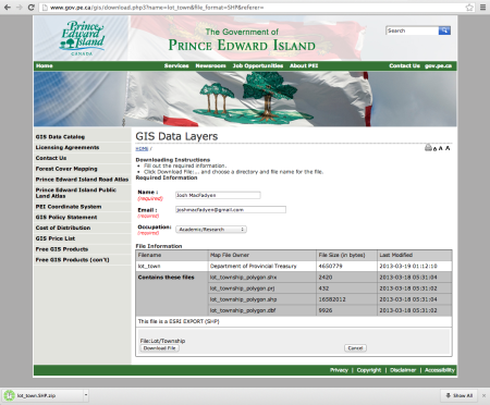
Figure 3
Add lot_township_polygon to QGIS:
- under Layer on the toolbar, choose Add Vector Layer (alternatively the same icon you see next to ‘Add Vector Layer’ can also be selected from the tool bar)
- Click Browse. Navigate to your unzipped file and select the file titled ‘lot_township_polygon.shp’
- Click Open

Figure 4
For more information on adding and visualizing layers see Installing QGIS 2.0 and adding Layers.
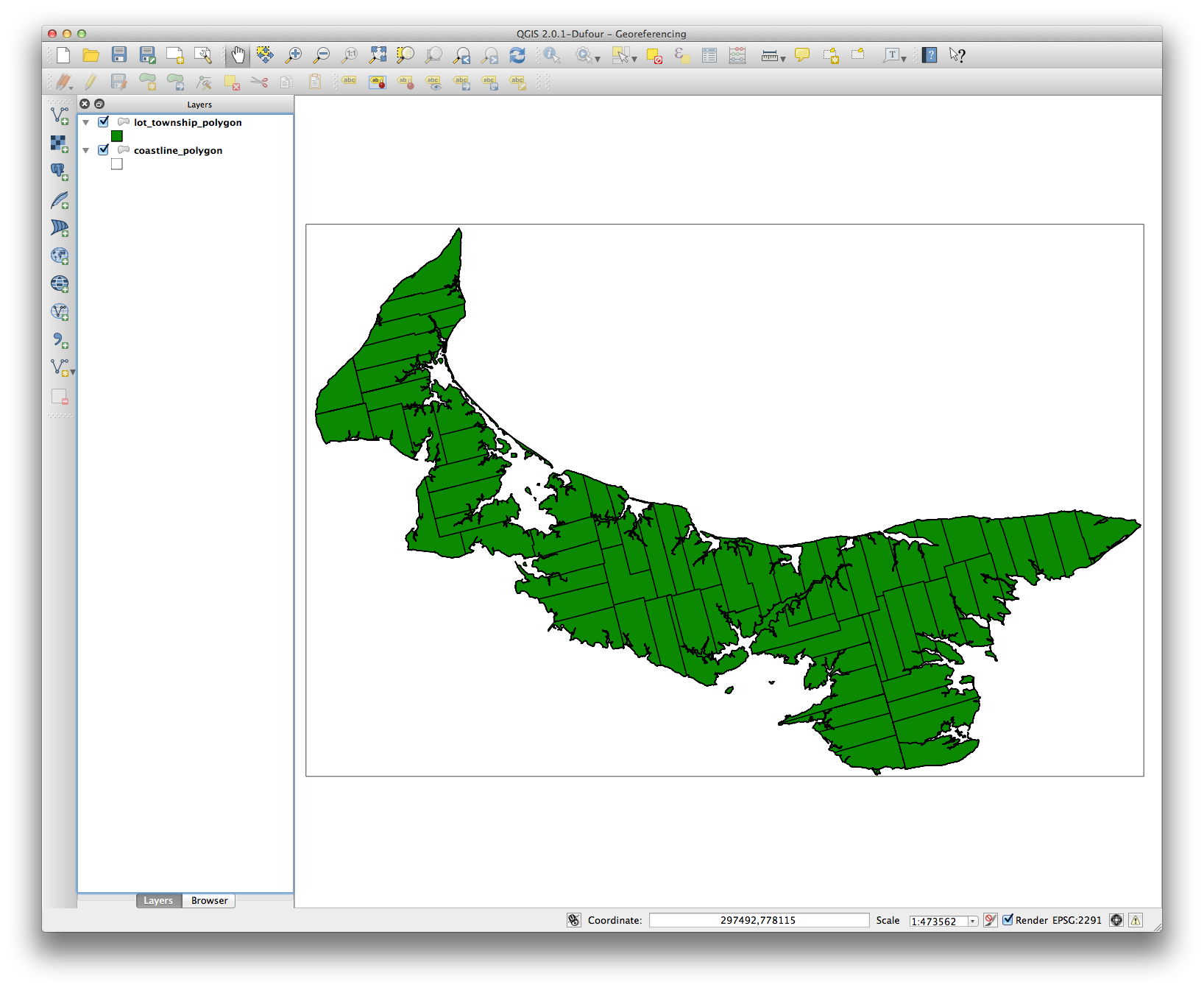
Figure 5
Open the Georeferencer Tool
Georeferencer is now available under the Raster menu on the toolbar – select it.
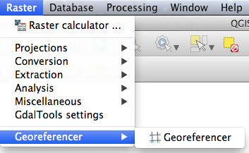
Figure 6
Add your historical map:
- In the resulting window, click on the Open Raster button on the top left (which looks identical to the Add Raster layer).

Figure 7
- Find the file titled ‘PEI_LakeMap1863.jpg’ on your computer and select Open (the file can be downloaded here or in its original location at the Island Imagined online map repository)
- You will be prompted to define this layer’s coordinate system. In the Filter box search for ‘2291′, then in the box below select ‘NAD83(CSRS98) / Prince Edward …’
The result will look like this:
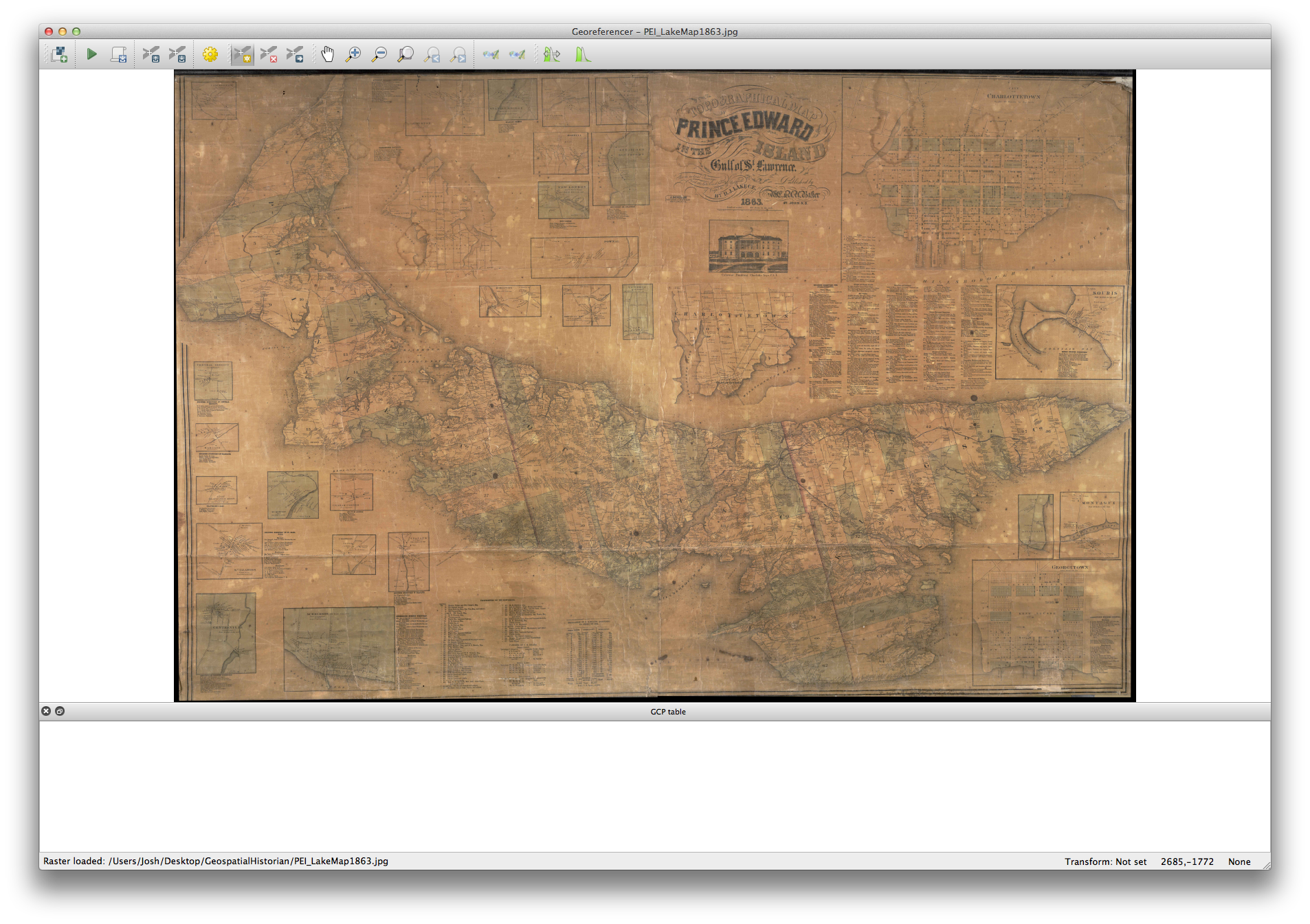
Figure 8
Adding control points:
Plan the locations you are going to use as control points in advance of the steps that follow. It is much easier to navigate around the historical map first, so get a good idea of the best points to use and keep them in mind.
Some tips for choosing control points:
- How many points do you need? Usually the more points you assign the more accurate your georeferenced map will be. Two control points will tell the GIS to scale and rotate the map to those two points, but in order to truly rubber-sheet the historical document you need to add more points.
- Where should you put control points? Select areas as close as possible to the four corners of your map so that these outer areas do not get omitted in the rubber-sheeting.
- Select additional control points close to your area of interest. Everything in between the four corner control points should georeference evenly, but if you are concerned about the accuracy of one place in particular, make sure to select additional control points in that area.
- Select the middle of intersections and roads, because the edges of roads changed a certain amount over time as road improvements were made.
- Check that your control points did not change location over time. Roads were often re-routed, and even houses and other buildings were moved, especially in Atlantic Canada!
Add your first control point:
First, navigate to the location of your first control point on the historical map.
- click on Zoom In Magnifying Glass on the window tool bar or use the mouse roller wheel to zoom in
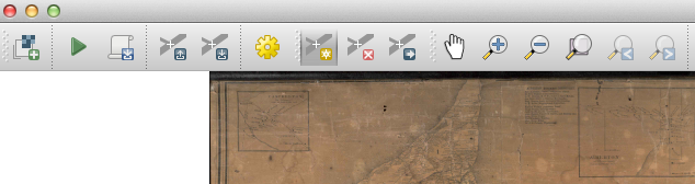
Figure 9
-
zoom in to a point which you can recognize on both your printed map and your GIS
-
Click on Add Point on toolbar
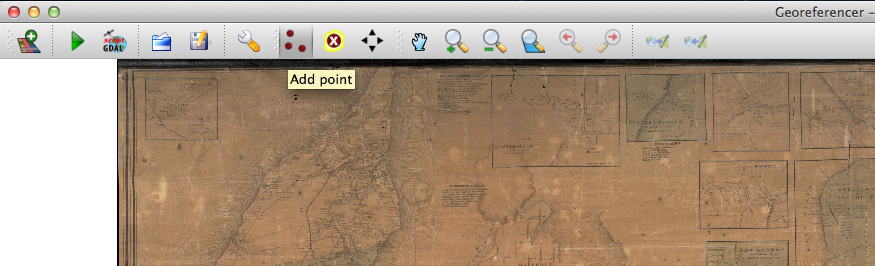
Figure 10
- Click on the place in the printed map that you can locate in your GIS (i.e. the control point). The Georeferencer window will now minimize automatically. If it does not (some versions have a bug in this plugin) manually minimize the window
- Click on the place in the GIS which matches the control point
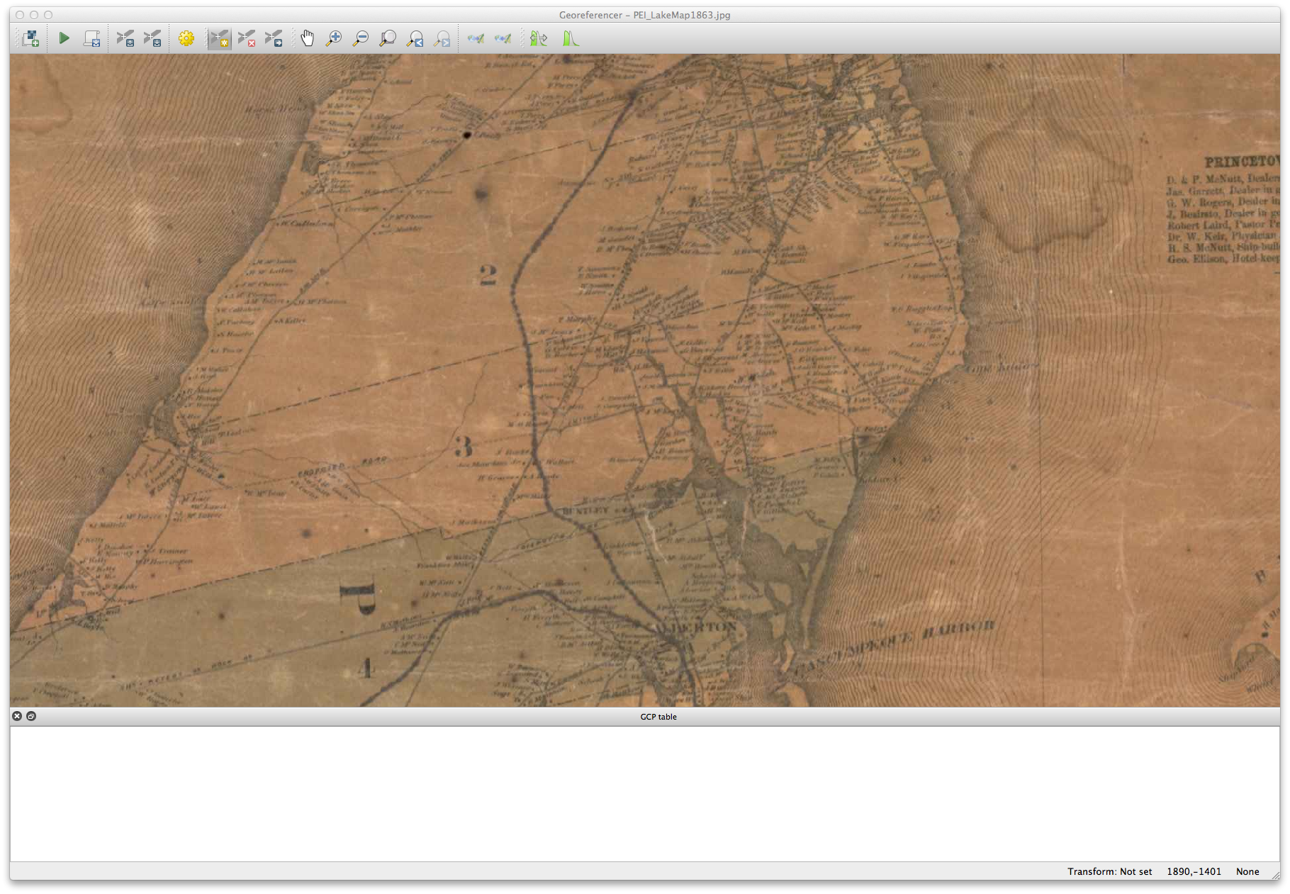
Figure 11
- At this stage we identified a problem in lot boundaries. We planned to use the location where the southern border of Lot 1 at the West end of the Province contains a “dog leg” near the middle of the land mass. However, it was clear that not all the dog legs on these lots matched the historical map. It is possible that lot boundaries have changed somewhat in the 250 years since they were established, so it is best to choose the point you are most sure of. In this case the dog leg between Lot 2 and Lot 3 was fine (see arrow). It was the border of Lots 3 and 4 that has changed. The discrepancy at the border of 1 and 2 shows that more control points are needed to properly rubber-sheet this somewhat distorted 1863 map to the Provincial GIS layer
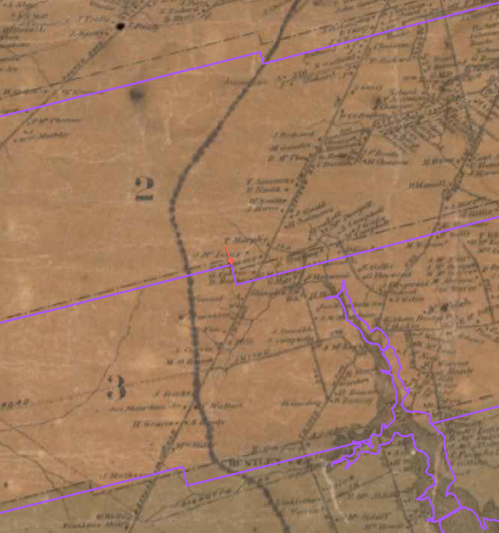
Figure 12
Add at least one more control point:
- return to the Georeferencer window and repeat the steps under ‘Add your first control point’ above, to add additional control points.
- Add a point close to the opposite side of your printed map (the further apart your control points are placed the more accurate the georeferencing process) and another one near Charlottetown
- return to the Georeferencer window. You should see three red dots on the printed map, and three records in the GCP table at the bottom of your window (outlined in red on the following image)
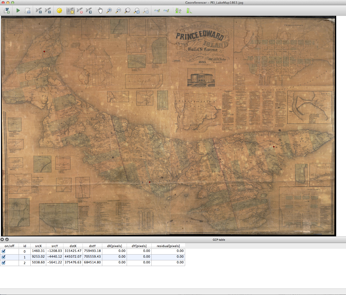
Figure 13
Determine the transformation settings:
Before you click Play and start the automated georeferencing process you need to tell QGIS where to save the new file (this will be a raster file), how it should interpret your control points, and how it should compress the image.
- Click on the Transformation Settings button

Figure 14
Most of these settings can be left as default: linear transformation type, nearest neighbour resampling method, and LZW compression. (The world file is not necessary, unless you want to georeference the same image again in another GIS or if someone else needs to georeference the image and does not have access to your GIS data, coordinate reference system, etc.) The target SRS is not important, but you could use this feature to give the new raster a different reference system.
- Assign a folder for your new georeferenced raster file. Tif is the default format for rasters georeferenced in QGIS.
- Be aware that a Tif file is going to be much larger than your original map, even with LZW compression, so make sure you have adequate space if you are using a jump drive. (warning: the Tif file produced from this 6.8 Mb .jpg will be over 1GB once georeferenced. One way to manage the size of the georeferenced raster file while maintaining a high enough resolution for legibility is to crop out only the area needed for the map project. In this case, a lower resolution option is also available from the Island Imagined online map repository.)
- Leave the target resolution at the default
- You can select ‘Use 0 transparency when needed’ to eliminate black spaces around the edges of the map, but this is not necessary and you can experiment as needed
- Make sure ‘Load in QGIS’ is selected to save a step. This will automatically add the new file to your GIS’s Table of Contents so that you don’t have to go looking for the Tif file later
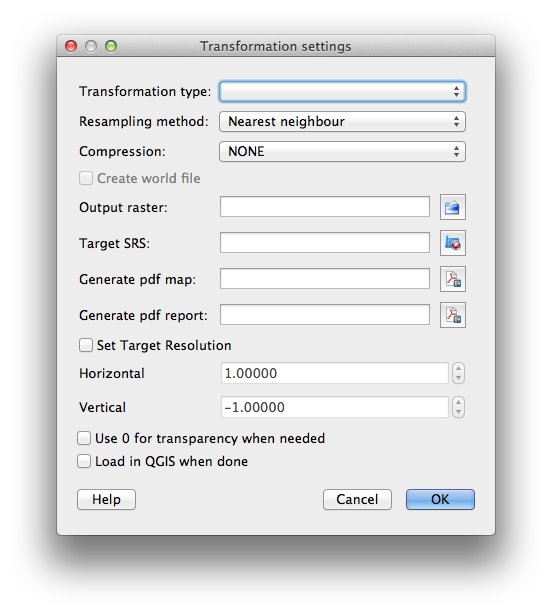
Figure 15
Georeference!
- Click on the Play button on the toolbar (beside Add Raster) – this begins the georeferencing process

Figure 16
Figure 17
- A window will appear titled Define CRS: select 2291, click OK
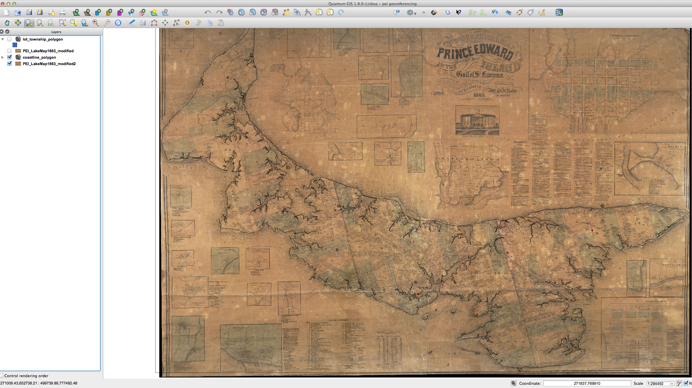
Figure 18
Explore your map:
- Drag the new layer ‘PEI_LakeMap1863_modified’ down to the bottom of your Table of Contents (i.e. below the ‘lot_township_polygon’ layer
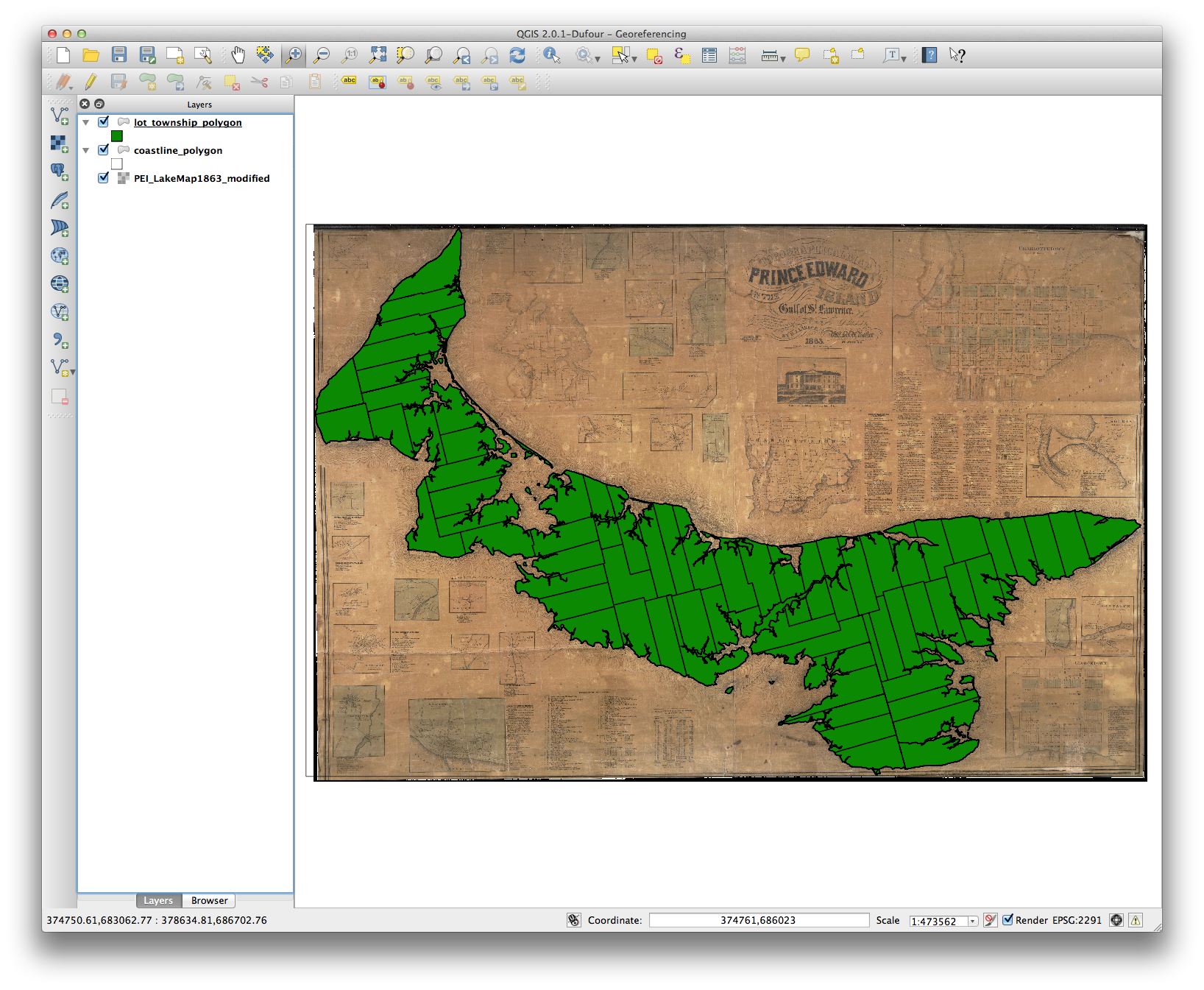
Figure 19
- Change the fill of the lot_township_polygon layer to ‘no brush’ by Selecting the layer, clicking on Layer -> Properties, and clicking on Symbol Properties. Click OK
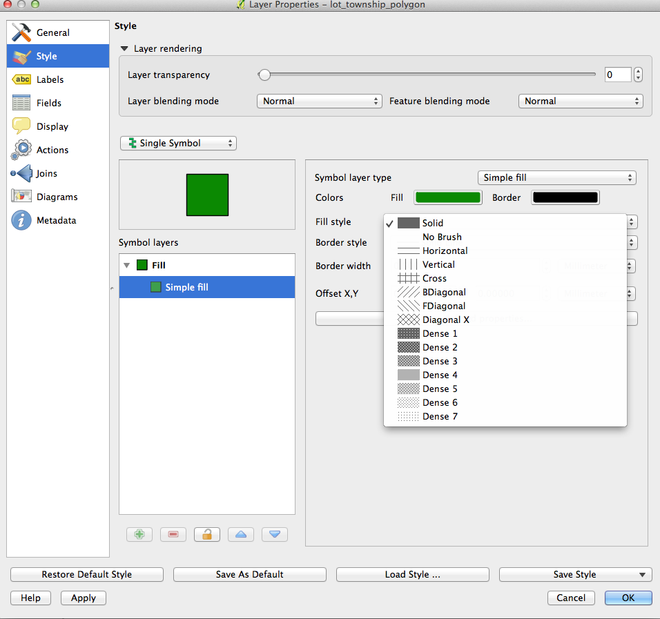
Figure 20
- Now you should see the modern GIS layer with the historical map in behind
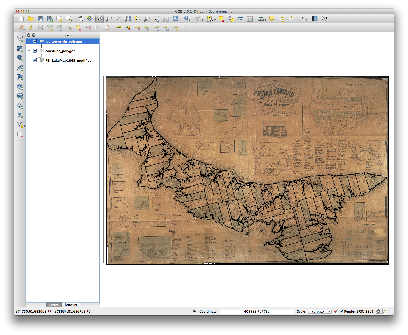
Figure 21
Now that you have a newly georeferenced map in your GIS you can explore the layer, adjust the transparency, contrast and brightness, and go back through Creating New Vector Layers in QGIS to digitize some of the historical information that you have created. For instance, this georeferenced map of PEI shows the locations of all homes in 1863, including the name of the head of household. By assigning points on the map you can enter home locations and owner names and then analyze or share that new geospatial layer as a shapefile.
By digitizing line vectors such as roads or coastlines you can compare the location of these features with other historical data, or simply compare them visually with the lot_township_polygon layer in this GIS.
In more advanced processes you can even drape this georeferenced image over a DEM (digital elevation model) to give it a hillshade terrain or 3D effect and perform a ‘fly-over’ of PEI homes in the nineteenth century.
This lesson is part of the Geospatial Historian.