
Contents
- Introduction
- Prerequisites
- Why K-Means clustering and DBSCAN?
- What is Clustering?
- How Does K-Means Work?
- How Many Clusters Should I Choose?
- How Does DBSCAN Work?
- First Case Study: Applying K-Means to the Ancient Authors Dataset from Brill’s New Pauly
- Second Case Study: Clustering Textual Data
- Summary
- Bibliography
- Footnotes
Introduction
This tutorial demonstrates how to implement and apply k-means clustering and DBSCAN in Python. K-means and DBSCAN are two popular clustering algorithms that can be used, in combination with others, during the exploratory data analysis to discover (hidden) structures in your data by identifying groups with similar features (see Patel 2019 in the bibliography). We will implement the clustering algorithms using scikit-learn, a widely applied and well-documented machine learning framework in Python. Also, scikit-learn has a huge community and offers smooth implementations of various machine learning algorithms. Once you have understood how to implement k-means and DBSCAN with scikit-learn, you can easily use this knowledge to implement other machine learning algorithms with scikit-learn, too.
This tutorial consists of two different case studies. The first case study clusters and analyzes an ancient authors dataset from Brill’s New Pauly. The second case study focuses on clustering textual data, namely abstracts of all published articles in the journal Religion (Taylor & Francis). These two datasets have been selected to illustrate how clustering algorithms can handle different data types (including numerical and textual features) and potentially be applied to a broad range of potential research topics.
The following section will introduce both datasets.
First Case Study: Ancient Authors in Brill’s New Pauly
In this example, we will use k-means to analyze a dataset including information about 238 ancient authors from Greco-Roman antiquity. The data was taken from the official Brill’s New Pauly website, and originates from Supplement I Volume 2: Dictionary of Greek and Latin Authors and Texts. Der Neue Pauly: Realenzyklopädie der Antike (in English Brill’s New Pauly) (1996–2002) is a well-known encyclopedia of the ancient world with contributions from established international scholars. It should be noted that access to the texts (and thus the data) in the New Pauly is not free of charge. I used my university’s access to obtain the data from the author entries. For the following analyses, I have not copied any texts from the New Pauly to the dataset. However, the numerical data in the dataset was extracted and partially accumulated from the author entries in the New Pauly. The original German version has been translated into English since 2002. I will refer to the text using its German abbreviation (DNP) from here onwards.
This tutorial demonstrates how k-means can help to cluster ancient authors into separate groups. The overall idea is that clustering algorithms either provide us with new insights into our data structure, or falsify/verify existing hypotheses. For instance, there might be groups of authors who are discussed at length but to whom few manuscripts are attributed. Meanwhile, other groups may include authors to whom many surviving manuscripts are ascribed but who only have short entries in the DNP. Another scenario could be that we find groups of authors associated with many early editions but only a few modern ones. This would point to the fact that modern scholars continue to rely on older editions when reading these authors. In the context of this tutorial, we will leave it to the algorithms to highlight such promising clusters for us.
The author data was collected from the official website using Python modules and libraries such as requests, BeautifulSoup, and pandas.1 The data was then stored in a csv file named DNP_ancient_authors.csv (see also the GitHub repository).
A single observation (row) in the DNP_ancient_authors.csv dataset contains an author name as an index and observations of the following seven features (variables):
- Word count of the entry in the DNP, used as a measure to evaluate the importance of the author (
word_count) - Number of modern translations (
modern_translations) - Number of known works (
known_works) - Number of existing manuscripts (
manuscripts) - Number of early editions (
early_editions) - Number of early translations (
early_translations) - Number of modern editions (
modern_editions) - Number of commentaries (
commentaries)
So, a single row in the dataset looks like this:
| authors | word_count | modern_translations | known_works | manuscripts | early_editions | early_translations | modern_editions | commentaries |
|---|---|---|---|---|---|---|---|---|
| Aelianus Tacticus | 350 | 1 | 1 | 0 | 3 | 6 | 1 | 0 |
Second Case Study: Article Abstracts in Religion (Journal)
The second dataset contains abstracts of all published articles in the journal Religion (Taylor & Francis). The abstracts were collected from the official website using Python modules and libraries such as requests, BeautifulSoup, and pandas. The data was stored in a csv file named RELIGION_abstracts.csv (see the GitHub repository). The current dataset includes abstracts from 701 articles published in 51 volumes between 1971–2021. However, some articles, particularly in older volumes, did not posses scrapable abstracts on the website and were thus left out. Other contribution types, including reviews and miscellanea, have also been excluded from this dataset.
A single row in the RELIGION_abstracts.csv dataset contains an numerical index and observations of the following four features (variables):
- The title of the article (
title) - The full abstract (
abstract) - A link to the article (
link) - A link to the volume in which the article (abstract) was published (
volume)
So, a single row in this dataset looks like this:
| title | abstract | link | volume |
|---|---|---|---|
| Norwegian Muslims denouncing terrorism: beyond ‘moderate’ versus ‘radical’? | In contemporary (…) | https://www.tandfonline.com/doi/full/10.1080/0048721X.2021.1865600 | https://www.tandfonline.com/loi/rrel20?treeId=vrrel20-51 |
The analysis in this tutorial focuses on clustering the textual data in the abstract column of the dataset. We will apply k-means and DBSCAN to find thematic clusters within the diversity of topics discussed in Religion. To do so, we will first create document vectors of each abstract (via Term Frequency - Inverted Document Frequency, or TF-IDF for short), reduce the feature space (which initially consists of the entire vocabulary of the abstracts), and then look for thematic clusters.
You can download both datasets as well as a Jupyter notebook containing the code we are writing in this tutorial from the GitHub repository. This lesson will work on any operating system, as long as you follow these instructions to set up an environment with Anaconda or Google Colab to run the Jupyter notebook locally or in the cloud. If you do not know how to set up a Jupyter notebook locally, this excellent PH tutorial might help you get started.
Prerequisites
To follow this tutorial, you should have basic programming knowledge (preferably Python) and be familiar with central Python libraries, such as pandas and matplotlib (or their equivalents in other programming languages). I also assume that you have basic knowledge of descriptive statistics. For instance, you should know what mean, standard deviation, and categorical/continuous variables are.
Why K-Means clustering and DBSCAN?
Generally, you can choose between several clustering algorithms to analyze your data, such as k-means clustering, hierarchical clustering, and DBSCAN. We focus on k-means clustering in this tutorial since it is a relatively easy-to-understand clustering algorithm with a fast runtime speed that still delivers decent results,2 which makes it an excellent model to start with. I have selected DBSCAN as the second clustering algorithm for this tutorial since DBSCAN is an excellent addition to k-means. Among other capabilities, DBSCAN allows you to focus on dense and non-linear clusters in your data while leaving noise points or outliers outside the dense clusters, which is something that k-means cannot do independently (k-means adds the noise points or outliers to the k-clusters).
However, implementing other clustering algorithms in combination with scikit-learn should be fairly straight-forward once you are familiar with the overall workflow. Thus, if you decide to analyze your data with additional clustering algorithms (such as hierarchical clustering), you can easily do so after finishing this tutorial. In general, it is advisable to apply more than one clustering algorithm to get different perspectives on your data and evaluate each model’s results.
What is Clustering?
Clustering is part of the larger field of machine learning. Machine learning is an artificial intelligence process by which computers can learn from data without being explicitly programmed (see Géron 2019, 2 in the bibliography), meaning that a machine learning model, once it is set up, can independently discover structures in the data or predict new (unknown) data. The field of machine learning can be separated into supervised, unsupervised, and reinforcement learning (see Géron 2019, 7-17 in the bibliography).
Supervised machine learning uses labeled data to train machine learning algorithms to make accurate predictions for new data. A good example is a spam filter (with emails either labeled as “spam” or “not-spam”). One way to assess a supervised machine learning model’s accuracy is to test it on some pre-labeled data, then compare the machine learning model’s labeling predictions with the original output. Among other things, the model’s accuracy depends on the quantity and quality of the labeled data it has been trained on and its parameters (hyperparameter tuning). Thus, building a decent supervised machine learning model involves a continuous loop of training, testing, and fine-tuning of the model’s parameters. Common examples of supervised machine learning classifiers are k-nearest neighbors (KNN) and logistic regression.
Unsupervised learning is applied to unlabeled data. Among other things, unsupervised learning is used for anomaly detection, dimensionality reduction, and clustering. When applying unsupervised machine learning algorithms, we do not feed our model with prelabeled data to make predictions for new data. Instead, we want the model to discern potential structures in our data. The datasets in this tutorial are a good example: we are only feeding our model either the author or abstract data, and we expect the model to indicate where (potential) clusters exist (for instance, articles in Religion with similar topics). Hyperparameter tuning can also be a part of unsupervised learning; however, in these cases, the results of the clustering cannot be compared to any prelabeled data. Yet, we can apply measures such as the so-called elbow method or the silhouette score to evaluate the model’s output based on different parameter choices (such as the n number of clusters in k-means).
Reinforcement learning is less relevant for scholars in the humanities. Reinforcement learning consists of setting up an agent (for instance, a robot) that performs actions and is either rewarded or punished for their execution. The agent learns how to react to its environment based on the feedback it received from its former actions.
How Does K-Means Work?
The following overview of the k-means algorithm focuses on the so-called naive k-means clustering, in which the cluster centers (so-called centroids) are randomly initialized. However, the scikit-learn implementation of k-means applied in this tutorial already integrates many improvements to the original algorithm. For instance, instead of randomly distributing the initial cluster centers (centroids), the scikit-learn model uses a different approach called k-means++, which is a smarter way to distribute the initial centroids. Yet, the way k-means++ works is beyond the scope of this tutorial, and I recommend reading this article by David Arthur and Sergei Vassilvitskii if you want to learn more.
The K-Means Algorithm
To explain how k-means works, let us review a snippet from our DNP_ancien_authors.csv dataset. Even though we will later include more features, it is helpful to focus on a few key features in this introductory section to explain how the clustering techniques work.
| authors | word_count | known_works |
|---|---|---|
| Aelianus Tacticus | 350 | 1 |
| Ambrosius | 1221 | 14 |
| Anacreontea | 544 | 1 |
| Aristophanes | 1108 | 11 |
To start with the k-means clustering, you first need to define the number of clusters you want to find in your data. In most cases, you will not know how many clusters exist in your data, so choosing the appropriate initial number of clusters is already a tricky question. We will address this issue below, but let us first review how k-means generally functions.
In our example, we will assume that we are trying to identify two clusters. The naive k-means algorithm will now initialize the model with two randomly distributed cluster centers in the two-dimensional space.
The main algorithm consists of two steps. The first step is to measure the distances between every data point and the current cluster centers (in our case, via Euclidean distance \( \sqrt[]{(x_1-x_2)^{2}+(y_1-y_2)^{2}} \), where \( (x_1,y_1) \) and \( (x_2,y_2) \) are two data points in our two-dimensional space). After measuring the distances between each data point and the cluster centers, every data point is assigned to its nearest cluster center.
The second step consists of creating new cluster centers by calculating the mean of all the data points assigned to each cluster.
After creating the new cluster centers, the algorithm starts again with the data points’ reassignment to the newly created cluster centers. The algorithm stops once the cluster centers are more or less stable. The Wikipedia entry on k-means clustering provides helpful visualizations of this two-step process.
The plotted results when clustering our snippet from the DNP_ancient_authors.csv dataset look like this, including the position of the final centroids:
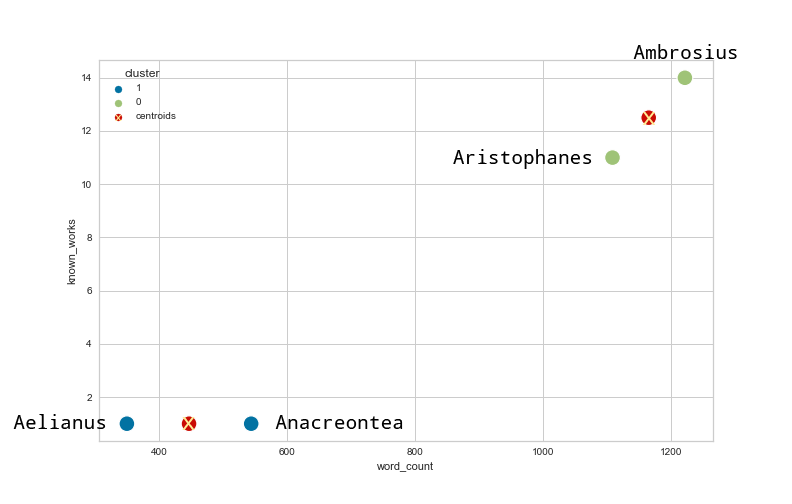
Figure 1: The clustered ancient authors data and the centroids using k-means in a two-dimensional space.
This appears satisfactory, and we can quickly see how the centroids are positioned between the data points that we intuitively assume to represent one cluster. However, we can already notice that the scales of both axes differ significantly. The y-axis ranges from 1–14, whereas the x-axis scale ranges from 300–1300. Thus, a change on the x-axis is likely to influence the distance between data points more significantly than a change on the y-axis. This, in turn, also impacts the placement of the centroids and thus the cluster building process. To showcase this problem, let us change the word count of Aristophanes from 1108 to 700.
| authors | word_count | known_works |
|---|---|---|
| Aelianus Tacticus | 350 | 1 |
| Ambrosius | 1221 | 14 |
| Anacreontea | 544 | 1 |
| Aristophanes | 700 | 11 |
If we apply k-means clustering on the changed dataset, we get the following result:
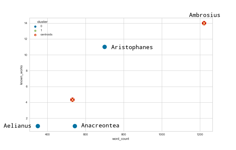
Figure 2: A new version of the clustered data and the centroids using k-means on the changed ancient authors data.
As you can see, a change of word count resulted in a new cluster of three authors who each have entries of approximately the same word count in the DNP, but who have a significantly different number of known published works. But does this really make sense? Wouldn’t it be more reasonable to leave Ambrosius and Aristophanes in the same cluster since they have both written approximately the same number of documented works? To account for such problems based on different scales, it is advisable to normalize the data before clustering it. There are different ways to do this, among them min-max normalization and z-score normalization, which is also called standardization. In this tutorial, we will focus on the latter. This means that we first subtract the mean from each data point and then divide it by the standard deviation of the data in the respective column. Fortunately, scikit-learn already provides us with implementations of these normalizations, so we do not have to calculate them manually.
The standardized (z-score) snippet of the ancient authors dataset looks like this:
| authors | word_count | known_works |
|---|---|---|
| Aelianus Tacticus | -1.094016 | -0.983409 |
| Ambrosius | 1.599660 | 1.239950 |
| Anacreontea | -0.494047 | -0.983409 |
| Aristophanes | -0.011597 | 0.726868 |
If we now apply a k-means clustering on the standardized dataset, we get the following result:
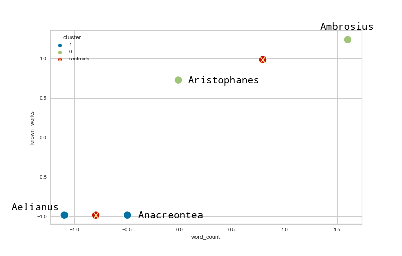
Figure 3: Using k-means clustering on the standardized dataset.
As you can see, changing the word count now has a less significant influence on the clustering. In our example, working with the standardized dataset results in a more appropriate clustering of the data since the known_works feature would otherwise lose much of its value for the overall analysis.
How Many Clusters Should I Choose?
Elbow Method
The question of how many cluster centers to choose is a difficult one. There is no one-size-fits-all solution to this problem. Yet, specific performance measures might help to select the right number of clusters for your data. A helpful example that we will be using in this tutorial is the elbow method. The elbow method is based on measuring the inertia of the clusters for different numbers of clusters. In this context, inertia is defined as:
Sum of squared distances of samples to their closest cluster center.3
The inertia decreases with the number of clusters. The extreme is that inertia will be zero when n is equal to the number of data points. But how could this help us find the right amount of clusters? Ideally, you would expect the inertia to decrease more slowly from a certain n onwards, so that a (fictional) plot of the inertia/cluster relation would look like this:
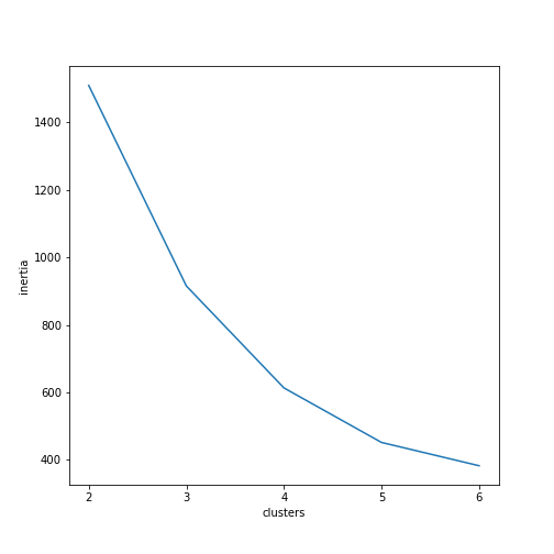
Figure 4: Fictional example of inertia for k clusters.
In this plot, the “elbow” is found at four clusters. This indicates that four clusters might be a reasonable trade-off between relatively low inertia (meaning the data points assigned to the clusters are not too far away from the centroids) and as few clusters as possible. Again, this method only provides you with an idea of where to start investigating. The final decision is up to you and highly depends on your data and your research question. Figuring out the right amount of clusters should also be accompanied by other steps, such as plotting your data or assessing other statistics. We will see how inertia helps us to discover the right amount of clusters for our DNP_ancient_authors.csv dataset in the following application of k-means.
Silhouette Score
Another possible way to evaluate the clustering of your data is to use the silhouette score, a method that allows you to assess how well each data point is associated with its current cluster. The way the silhouette score works is very well described in the Wikipedia article “Silhouette (clustering)”:
The silhouette value is a measure of how similar an object is to its own cluster (cohesion) compared to other clusters (separation). The silhouette ranges from −1 to +1, where a high value indicates that the object is well matched to its own cluster and poorly matched to neighboring clusters. If most objects have a high value, then the clustering configuration is appropriate. If many points have a low or negative value, then the clustering configuration may have too many or too few clusters.
In this tutorial, we will be using the silhouette scores with the machine learning visualization library yellowbrick in Python. Plotting the average silhouette score of all data points against the silhouette score of each data point in a cluster can help you to evaluate the quality of your model and the suitability of your current choice of parameter values.
To illustrate how a silhouette plot can help you find the correct number of clusters for your data, we can take a dummy example from our ancient author dataset. The data is based on a fictive sample of the number of known works and the word count of selected authors. The data has already been standardized using the z-score.
| authors | known_works | word_count |
|---|---|---|
| Author A | 0.24893051 | 0.83656758 |
| Author B | 0.38169345 | 0.04955707 |
| Author C | 0.11616757 | 0.34468601 |
| Author D | -0.01659537 | 0.14793338 |
| Author E | -1.21146183 | -1.18014685 |
| Author F | -1.07869889 | -1.27852317 |
| Author G | -0.94593595 | -1.22933501 |
| Author H | -1.07869889 | -1.1309587 |
| Author I | -0.68041007 | -0.34394819 |
| Author J | -0.81317301 | -0.83582976 |
| Author K | -0.41488419 | -0.54070081 |
| Author L | -0.54764713 | -0.43838945 |
| Author M | 1.1782711 | 1.62357809 |
| Author N | 1.31103404 | 1.52520177 |
| Author O | 1.57655992 | 1.41698783 |
| Author P | 1.97484874 | 1.03332021 |
We can now plot the silhouette score for different cluster numbers n. In this example, we will plot the silhouette scores for two, three, and four clusters using k-means.
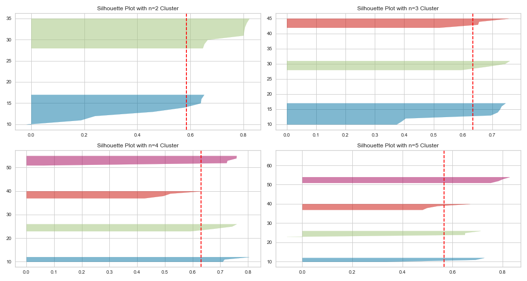
Figure 5: Silhouette plots using k-means with n clusters between two and five.
The vertical dashed line indicates the average silhouette score of all data points. The horizontal “knives” represent an overview of all data points in a cluster and their individual silhouette scores in descending order (from top to bottom). The silhouette plots show us that a cluster number between four and five seems to be most appropriate for our dataset. Particularly the data points with n=4 clusters have a relatively high average silhouette score (over 0.6), and the cluster “knives” seem to have approximately the same size and are not too sharp, which indicates that the cohesion within each cluster is not too bad. Indeed, if we plot our data using k-means with n=4 clusters, we can see that this choice is a reasonable cluster number for our dataset and offers a good impression of the overall distribution of the data points.
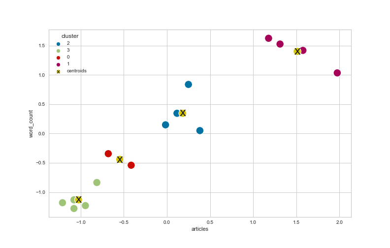
Figure 6: Scatterplot of the dataset using k-means clustering with n=4 clusters.
How Does DBSCAN Work?
DBSCAN is short for “Density-Based Spatial Clustering of Applications with Noise.” Unlike the k-means algorithm, DBSCAN does not try to cluster every single data point in a dataset. Instead, DBSCAN looks for dense regions of data points in a set while classifying data points without any direct neighbors as outliers or ‘noise points’. DBSCAN can be a great choice when dealing with datasets that are not linearly clustered but still include dense regions of data points.
The DBSCAN Algorithm
The basic DBSCAN algorithm is very well explained in the corresponding wikipedia article.
- The first step consists of defining an ε-distance (eps) that defines the neighborhood region (radius) of a data point. Just as in the case of k-means-clustering, scikit-learn’s DBSCAN implementation uses Euclidean distance as the standard metric to calculate distances between data points. The second value that needs to be defined is the minimum number of data points that should be located in the neighborhood of data point to define its region as dense (including the data point itself).
- The algorithm starts by choosing a random data point in the dataset as a starting point. DBSCAN then looks for other data points within the ε-region around the starting point. Suppose there are at least n datapoints (with n equals the minimum number of data points specified before) in the neighborhood (including the starting point). In that case, the starting point and all the data points in the ε-region of the starting point are defined as core points that define a core cluster. If there are less than n data points found in the starting point’s neighborhood, the datapoint is labeled as an noise point or outlier (yet, it might still become a member of another cluster later on). In this case, the algorithm continues by choosing another unlabeled data point from the dataset and restarts the algorithm at step 2.
- If an initial cluster is found, the DBSCAN algorithm analyzes the ε-region of each core point in the initial cluster. If a region includes at least n data points, new core points are created, and the algorithm continues by looking at the neighborhood of these newly assigned core points, and so on. If a core point has less than n data points, some of which are still unlabeled, they will also be included in the cluster (as so-called border points). In cases where border points are part of different clusters, they will be associated with the nearest cluster
- Once every datapoint has been visited and labeled as either part of a cluster or as a noise point or outlier, the algorithm stops.
Unlike the k-means algorithm, the difficulty does not lie in finding the right amount of clusters to start with but in figuring out which ε-region is most appropriate for the dataset. A helpful method for finding the proper eps value is explained in this article on towardsdatascience.com. In short, DBSCAN enables us to plot the distance between each data point in a dataset and itentify its nearest neighbor. It is then possible to sort by distance in ascending order. Finally, we can look for the point in the plot which initiates the steepest ascent and make a visual evaluation of the eps value, similar to the ‘elbow’ evaluation method described above in the case of k-means)’. We will use this method later in this tutorial.
Now that we know how our clustering algorithms generally work and which methods we can apply to settle on the right amount of clusters let us apply these concepts in the context of our datasets from Brill’s New Pauly and the journal Religion. We will start by analyzing the DNP_ancient_authors.csv dataset.
First Case Study: Applying K-Means to the Ancient Authors Dataset from Brill’s New Pauly
1. Exploring the Dataset
Before starting with the clustering, we will explore the data by loading DNP_ancient_authors.csv into Python with pandas. Next, we will print out the first five rows and look at some information and overview statistics about each dataset using pandas’ info() and describe() methods.
import pandas as pd

# load the authors dataset that has been stored as a .csv files in a folder called "data" in the same directory as the Jupyter Notebook
df_authors = pd.read_csv("data/DNP_ancient_authors.csv", index_col="authors").drop(columns=["Unnamed: 0"])

# display dataset structure with the pandas .info() method
print(df_authors.info())

# show first 5 rows
print(df_authors.head(5))

# display some statistics
print(df_authors.describe())
The output of the info() method should look like this:
<class 'pandas.core.frame.DataFrame'>
Index: 238 entries, Achilles Tatius of Alexandria to Zosimus
Data columns (total 8 columns):
 #   Column               Non-Null Count  Dtype
---  ------               --------------  -----
 0   word_count           238 non-null    int64
 1   modern_translations  238 non-null    int64
 2   known_works          238 non-null    int64
 3   manuscripts          238 non-null    int64
 4   early_editions       238 non-null    int64
 5   early_translations   238 non-null    int64
 6   modern_editions      238 non-null    int64
 7   commentaries         238 non-null    int64
dtypes: int64(8)
memory usage: 16.7+ KB
As we can see, our data consists of 238 entries of type integer. Next, we will examine our data through the output of the pandas describe() method.
The output of df_authors.describe() should look like this:
word_count	modern_translations	known_works	manuscripts	early_editions	early_translations	modern_editions	commentaries
count	238.000000	238.000000	238.000000	238.000000	238.000000	238.000000	238.000000	238.000000
mean	904.441176	12.970588	4.735294	4.512605	5.823529	4.794118	10.399160	3.815126
std	804.388666	16.553047	6.784297	4.637702	4.250881	6.681706	11.652326	7.013509
min	99.000000	0.000000	0.000000	0.000000	0.000000	0.000000	0.000000	0.000000
25%	448.750000	4.250000	1.000000	1.000000	3.000000	0.000000	4.000000	0.000000
50%	704.000000	9.000000	2.000000	3.000000	5.000000	2.500000	7.000000	1.000000
75%	1151.500000	15.750000	6.000000	6.000000	8.000000	8.000000	14.000000	4.000000
max	9406.000000	178.000000	65.000000	34.000000	28.000000	39.000000	115.000000	43.000000
We can see that the standard deviation and the mean values vary significantly between the word_count column and the other columns. When working with metrics such as Euclidean distance in the k-means algorithm, different scales between the columns can become problematic. Thus, we should standardize the data before applying the clustering algorithm.
Furthermore, we have an significant standard deviation in almost every column and a vast difference between the 75th percentile value and the maximum value, particularly in the word_count column. This indicates that we might have some noise in our dataset, and it might be necessary to get rid of the noisy data points before we continue with our analysis. Therefore, we only keep those data points in our data frame with a word count within the 90th percentile range.
ninety_quantile = df_authors["word_count"].quantile(0.9)
df_authors = df_authors[df_authors["word_count"] <= ninety_quantile]
2. Imports and Additional Functions
Before we start with the actual clustering process, we first import all the necessary libraries and write a couple of functions that will help us to plot our results during the analysis. We will also use these functions and imports during the second case study in this tutorial (analyzing the Religion abstracts data). Thus, if you decide to skip the analysis of the ancient authors data, you still need to import these functions and libraries to execute the code in the second part of this tutorial.
from sklearn.preprocessing import StandardScaler as SS # z-score standardization
from sklearn.cluster import KMeans, DBSCAN # clustering algorithms
from sklearn.decomposition import PCA # dimensionality reduction
from sklearn.metrics import silhouette_score # used as a metric to evaluate the cohesion in a cluster
from sklearn.neighbors import NearestNeighbors # for selecting the optimal eps value when using DBSCAN
import numpy as np

# plotting libraries
import matplotlib.pyplot as plt
import seaborn as sns
from yellowbrick.cluster import SilhouetteVisualizer
The following function will help us to plot (and save) the silhouette plots.
def silhouettePlot(range_, data):
    '''
    we will use this function to plot a silhouette plot that helps us to evaluate the cohesion in clusters (k-means only)
    '''
    half_length = int(len(range_)/2)
    range_list = list(range_)
    fig, ax = plt.subplots(half_length, 2, figsize=(15,8))
    for _ in range_:
        kmeans = KMeans(n_clusters=_, random_state=42)
        q, mod = divmod(_ - range_list[0], 2)
        sv = SilhouetteVisualizer(kmeans, colors="yellowbrick", ax=ax[q][mod])
        ax[q][mod].set_title("Silhouette Plot with n={} Cluster".format(_))
        sv.fit(data)
    fig.tight_layout()
    fig.show()
    fig.savefig("silhouette_plot.png")
The next function will help us to plot (and save) the elbow plots.
def elbowPlot(range_, data, figsize=(10,10)):
    '''
    the elbow plot function helps to figure out the right amount of clusters for a dataset
    '''
    inertia_list = []
    for n in range_:
        kmeans = KMeans(n_clusters=n, random_state=42)
        kmeans.fit(data)
        inertia_list.append(kmeans.inertia_)

    # plotting
    fig = plt.figure(figsize=figsize)
    ax = fig.add_subplot(111)
    sns.lineplot(y=inertia_list, x=range_, ax=ax)
    ax.set_xlabel("Cluster")
    ax.set_ylabel("Inertia")
    ax.set_xticks(list(range_))
    fig.show()
    fig.savefig("elbow_plot.png")
The next function assists us in finding the right eps value when using DBSCAN.
def findOptimalEps(n_neighbors, data):
    '''
    function to find optimal eps distance when using DBSCAN; based on this article: https://towardsdatascience.com/machine-learning-clustering-dbscan-determine-the-optimal-value-for-epsilon-eps-python-example-3100091cfbc
    '''
    neigh = NearestNeighbors(n_neighbors=n_neighbors)
    nbrs = neigh.fit(data)
    distances, indices = nbrs.kneighbors(data)
    distances = np.sort(distances, axis=0)
    distances = distances[:,1]
    plt.plot(distances)
The last function progressiveFeatureSelection() implements a basic algorithm to select features from our dataset based on the silhouette score and k-means clustering. The algorithm first identifies a single feature with the best silhouette score when using k-means clustering. Afterward, the algorithm trains a k-means instance for each combination of the initially chosen feature and one of the remaining features. Next, it selects the two-feature combination with the best silhouette score. The algorithm uses this newly discovered pair of features to find the optimal combination of these two features with one of the remaining features, and so on. The algorithm continues until it has discovered the optimal combination of n features (where n is the value of the max_features parameter).
The algorithm is inspired by this discussion on stackexchange.com. Yet, don’t worry too much about this implementation; there are better solutions for feature selection algorithms out there, as shown in in Manoranjan Dash and Huan Liu’s paper ‘Feature Selection for Clustering’ and Salem Alelyani, Jiliang Tang, and Huan Liu’s ‘Feature Selection for Clustering: A Review’. However, most of the potential algorithms for feature selection in an unsupervised context are not implemented in scikit-learn, which is why I have decided to implement one myself, albeit basic.
def progressiveFeatureSelection(df, n_clusters=3, max_features=4,):
    '''
    very basic implementation of an algorithm for feature selection (unsupervised clustering); inspired by this post: https://datascience.stackexchange.com/questions/67040/how-to-do-feature-selection-for-clustering-and-implement-it-in-python
    '''
    feature_list = list(df.columns)
    selected_features = list()
    # select starting feature
    initial_feature = ""
    high_score = 0
    for feature in feature_list:
        kmeans = KMeans(n_clusters=n_clusters, random_state=42)
        data_ = df[feature]
        labels = kmeans.fit_predict(data_.to_frame())
        score_ = silhouette_score(data_.to_frame(), labels)
        print("Proposed new feature {} with score {}". format(feature, score_))
        if score_ >= high_score:
            initial_feature = feature
            high_score = score_
    print("The initial feature is {} with a silhouette score of {}.".format(initial_feature, high_score))
    feature_list.remove(initial_feature)
    selected_features.append(initial_feature)
    for _ in range(max_features-1):
        high_score = 0
        selected_feature = ""
        print("Starting selection {}...".format(_))
        for feature in feature_list:
            selection_ = selected_features.copy()
            selection_.append(feature)
            kmeans = KMeans(n_clusters=n_clusters, random_state=42)
            data_ = df[selection_]
            labels = kmeans.fit_predict(data_)
            score_ = silhouette_score(data_, labels)
            print("Proposed new feature {} with score {}". format(feature, score_))
            if score_ > high_score:
                selected_feature = feature
                high_score = score_
        selected_features.append(selected_feature)
        feature_list.remove(selected_feature)
        print("Selected new feature {} with score {}". format(selected_feature, high_score))
    return selected_features
Note that we have selected n=3 clusters as default for the k-means instance in progressiveFeatureSelection(). In the context of an advanced hyperparameter tuning (which is beyond the scope of this tutorial), it might make sense to train the progressiveFeatureSelection() with different n values for the k-means instance as well. For the sake of simplicity, we stick to n=3 clusters in this tutorial.
3. Standardizing the DNP Ancient Authors Dataset
Next, we initialize scikit-learn’s StandardScaler() to standardize our data. We apply scikit-learn’s StandardScaler() (z-score) to cast the mean of the columns to approximately zero and the standard deviation to one, to account for the huge differences between the word_count and the other columns in df_ancient_authors.csv.
scaler = SS()
DNP_authors_standardized = scaler.fit_transform(df_authors)
df_authors_standardized = pd.DataFrame(DNP_authors_standardized, columns=["word_count_standardized", "modern_translations_standardized", "known_works_standardized", "manuscripts_standardized", "early_editions_standardized", "early_translations_standardized", "modern_editions_standardized", "commentaries_standardized"])
df_authors_standardized = df_authors_standardized.set_index(df_authors.index)
4. Feature Selection
If you were to cluster the entire DNP_ancient_authors.csv with k-means, you would not find any reasonable clusters in the dataset. This is frequently the case when working with real-world data. However, in such cases, it might be pertinent to search for subsets of features that help us to structure the data. As we are only dealing with ten features, we could theoretically do this manually. However, because we have already implemented a basic algorithm to help us find potentially interesting combinations of features, we can also use our progressiveFeatureSelection() function. In this tutorial, we will search for three features that might be interesting to look at. Yet, feel free to try out different max_features with the progressiveFeatureSelection() function (as well as n_clusters). The selection of only three features (as well as n=3 clusters for the k-means instance) was a random choice which unexpectedly led to some exciting results; however, this does not mean that there are no other promising combinations which might be worth examining.
selected_features = progressiveFeatureSelection(df_authors_standardized, max_features=3, n_clusters=3)
Running this function, it turns out that the three features known_works_standardized, commentaries_standardized, and modern_editions_standardized might be worth considering when trying to cluster our data. Thus, we next create a new data frame with only these three features.
df_standardized_sliced = df_authors_standardized[selected_features]
5. Choosing the Right Amount of Clusters
We will now apply the elbow method and then use silhouette plots to obtain an impression of how many clusters we should choose to analyze our dataset. We will check for two to ten clusters. Note, however, that the feature selection was also made with a pre-defined k-means algorithm using n=3 clusters. Thus, our three selected features might already tend towards this number of clusters.
elbowPlot(range(1,11), df_standardized_sliced)
The elbow plot looks like this:
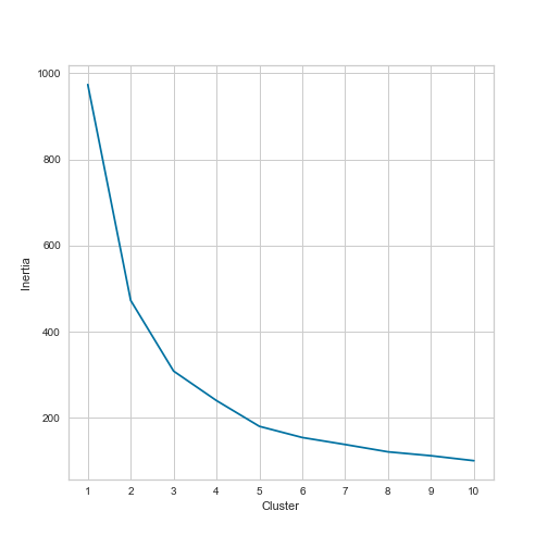
Figure 7: Elbow plot of the df_standardized_sliced dataset.
Looking at the elbow plot indeed shows us that we find an “elbow” at n=3 as well as n=5 clusters. Yet, it is still quite challenging to decide whether to use three, four, five, or even six clusters. Therefore, we should also look at the silhouette plots.
silhouettePlot(range(3,9), df_standardized_sliced)
The silhouette plots look like this:
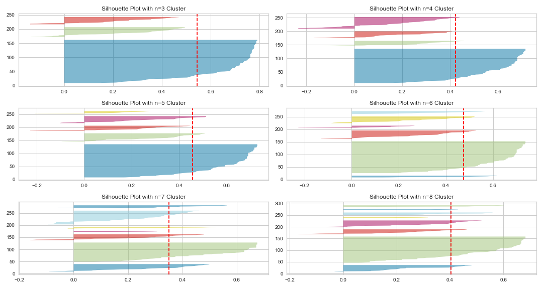
Figure 8: Silhouette plots of the df_standardized_sliced dataset.
Looking at the silhouette scores underlines our previous intuition that a selection of n=3 or n=5 seems to be the right choice of clusters. The silhouette plot with n=3 clusters in particular has a relatively high average silhouette score. Yet, because the two other clusters are far below the average silhouette score for n=3 clusters, we decide to analyze the dataset with k-means using n=5 clusters. However, the different sizes of the “knives” and their sharp form in both n=3 and n=5 clusters indicate a single dominant cluster and a couple of rather small and less cohesive clusters.
6. n=5 K-Means Analysis of the DNP Ancient Authors Dataset
Eventually, we can now train a k-means instance with n=5 clusters and plot the results using seaborn. I prefer plotting in two dimensions in Python, so we will use PCA() (Principal Component Analysis) to reduce the dimensionality of our dataset to two dimensions. PCA is a great way to reduce the dimensionality of a dataset while keeping the variance from higher dimensions.
PCA allows us to reduce the dimensionality of the original data substantially while retaining most of the salient information. On the PCA-reduced feature set, other machine learning algorithms—downstream in the machine learning pipeline—will have an easier time separating the data points in space (to perform tasks such as anomaly detection and clustering) and will require fewer computational resources. (quote from the online version of Ankur A. Patel: Hands-On Unsupervised Learning Using Python, O’Reilly Media 2020)
PCA can be used to reduce high-dimensional datasets for computational reasons. Yet, in this context, we only use PCA to plot the clusters in our dataset in a two-dimensional space. We will also apply PCA in the following text clustering. One huge disadvantage of using PCA is that we lose our initial features and create new ones that are somewhat nebulous to us, as they do not allow us to look at specific aspects of our data anymore (such as word counts or known works).
Before using PCA and plotting the results, we will instantiate a k-means instance with n=5 clusters and a random_state of 42. The latter parameter allows us to reproduce our results. 42 is an arbitrary choice here that refers to “Hitchhiker’s Guide to the Galaxy”, but you can choose whichever number you like.
kmeans = KMeans(n_clusters=5, random_state=42)
cluster_labels = kmeans.fit_predict(df_standardized_sliced)
df_standardized_sliced["clusters"] = cluster_labels

# using PCA to reduce the dimensionality
pca = PCA(n_components=2, whiten=False, random_state=42)
authors_standardized_pca = pca.fit_transform(df_standardized_sliced)
df_authors_standardized_pca = pd.DataFrame(data=authors_standardized_pca, columns=["pc_1", "pc_2"])
df_authors_standardized_pca["clusters"] = cluster_labels

# plotting the clusters with seaborn
sns.scatterplot(x="pc_1", y="pc_2", hue="clusters", data=df_authors_standardized_pca)
In the corresponding plot (see figure 9), we can clearly distinguish several clusters in our data. However, we also perceive what was already visible in the silhouette plots, namely that we only have one dense cluster and two to three less cohesive ones with several noise points.
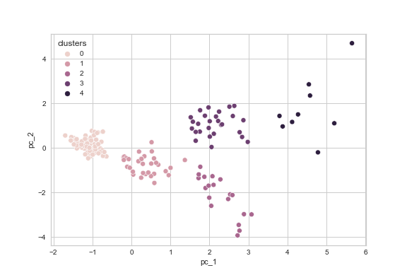
Figure 9: Final plot of the clustered df_standardized_sliced dataset with seaborn.
7. Conclusion
We were able to observe some clear clusters in our data when using known_works_standardized, commentaries_standardized, and modern_editions_standardized as a feature subset. But what does this actually tell us? This is a question that the algorithm cannot answer. The clustering algorithms only demonstrate that there are specific clusters under certain conditions, in this case, when looking for n=5 clusters with k-means and the above-mentioned subset of features. But what are these clusters about? Do they grant us valuable insights into our data? To answer this question, we need to look at the members of each cluster and analyze whether their grouping hints at certain aspects that might be worth exploring further.
In our example, looking at cluster 0 (the dense one in the left part of our plot) reveals that this cluster includes authors with very few known works, few to no commentaries, few modern editions, and rather short entries in the DNP (average word count of 513). Consequently, it largely consists of relatively unknown ancient authors.
| authors | word_count | modern_translations | known_works | manuscripts | early_editions | early_translations | modern_editions | commentaries |
|---|---|---|---|---|---|---|---|---|
| Achilles Tatius of Alexandria | 383 | 5 | 1 | 2 | 3 | 9 | 2 | 1 |
| Aelianus Tacticus | 350 | 1 | 1 | 0 | 3 | 6 | 1 | 0 |
| Aelianus, Claudius (Aelian) | 746 | 8 | 3 | 6 | 10 | 8 | 7 | 0 |
| Aeneas Tacticus | 304 | 5 | 1 | 1 | 1 | 2 | 6 | 0 |
| Aesop | 757 | 18 | 1 | 6 | 10 | 2 | 11 | 1 |
| Agatharchides of Cnidus | 330 | 2 | 3 | 0 | 4 | 1 | 1 | 0 |
| Agathias | 427 | 4 | 2 | 1 | 2 | 4 | 6 | 0 |
| Alexander of Tralleis | 871 | 4 | 4 | 7 | 3 | 3 | 4 | 2 |
| Ammianus Marcellinus | 573 | 8 | 1 | 3 | 6 | 4 | 6 | 6 |
| Anacreontea | 544 | 3 | 1 | 0 | 1 | 10 | 5 | 0 |
As we can see in this snippet that shows the first ten entries in cluster 0, the author names (except Aesop) are more or less supporting our initial assumption that we are predominately dealing with authors whose work is produced in few modern editions, particularly compared to the authors in cluster 4.
The authors in cluster 4 (the less cohesive cluster at the upper right of our plot) comprise well-known and extensively discussed authors including Plato or Aristophanes, who have all written several works that are still famous and have remained relevant over the centuries, demonstrated by the high number of modern editions and commentaries.
| authors | word_count | modern_translations | known_works | manuscripts | early_editions | early_translations | modern_editions | commentaries |
|---|---|---|---|---|---|---|---|---|
| Aeschylus of Athens | 1758 | 31 | 7 | 5 | 10 | 14 | 15 | 20 |
| Aristophanes of Athens | 1108 | 18 | 11 | 2 | 6 | 30 | 7 | 18 |
| Lucanus, Marcus Annaeus | 1018 | 17 | 1 | 11 | 8 | 15 | 20 | 25 |
| Plato | 1681 | 31 | 18 | 5 | 5 | 0 | 10 | 20 |
| Plutarchus of Chaeronea (Plutarch) | 1485 | 37 | 2 | 2 | 6 | 0 | 15 | 42 |
| Propertius, Sextus | 1443 | 22 | 1 | 5 | 5 | 5 | 24 | 22 |
| Sallustius Crispus, Gaius (Sallust) | 1292 | 17 | 5 | 12 | 7 | 15 | 15 | 16 |
| Sophocles | 1499 | 67 | 8 | 4 | 5 | 0 | 14 | 18 |
| Tacitus, (Publius?) Cornelius | 1504 | 29 | 5 | 6 | 10 | 14 | 31 | 20 |
If you want to have a closer look at the other clusters, I advise you to check out the Jupyter notebook in the GitHub repository.
Thus, our clustering of the DNP_ancient_authors.csv dataset has resulted in some promising clusters, which might help us develop new research questions. For instance, we could now take these clusters and apply our hypothesis about their relevance to further explore clustering the authors, based on their early and modern translations/editions. However, this is beyond the scope of this tutorial, which is primarily concerned with introducing tools and methods to examine such research questions.
Second Case Study: Clustering Textual Data
The second section of this tutorial will deal with textual data, namely all abstracts scraped from the Religion (journal) website. We will try to cluster the abstracts based on their word features in the form of TF-IDF vectors (which is short for “Term Frequency - Inverted Document Frequency”).
1. Loading the Dataset & Exploratory Data Analysis
Using a similar method as that used to analyze the DNP_ancient_authors.csv dataset, we will first load the RELIGION_abstracts.csv into our program and look at some summary statistics.
df_abstracts = pd.read_csv("data/RELIGION_abstracts.csv").drop(columns="Unnamed: 0")
df_abstracts.info()
df_abstracts.describe()
The result of the describe() method should print out something like this:
title	abstract	link	volume
count	701	701	701	701
unique	701	701	701	40
top	From locality to (...) https://www.tandfonline.com/doi/abs/10.1006/reli.1996.9998 Titel anhand dieser DOI in Citavi-Projekt übernehmen	https://www.tandfonline.com/loi/rrel20?treeId=vrrel20-50
freq	1	1	1	41
Unlike in the previous dataset, we are now dealing with features where every single observation is unique.
2. TF-IDF Vectorization
In order to process the textual data with clustering algorithms, we need to convert the texts into vectors. For this purpose, we are using the scikit-learn implementation of TF-IDF vectorization. For a good introduction to how TF-IDF works, see this great tutorial by Melanie Walsh.
Optional Step: Lemmatization
As an optional step, I have implemented a function called lemmatizeAbstracts() that groups, or ‘lemmatizes’ the abstracts using spaCy. Considering that we are not interested in stylistic similarities between the abstracts, this step helps to reduce the overall amount of features (words) in our dataset. As part of the lemmatization function, we also clean the text of all punctuation and other noise such as brackets. In the following analysis, we will continue working with the lemmatized version of the abstracts. However, you can also keep using the original texts and skip the lemmatization, although this might lead to different results.
# lemmatization (optional step)
import spacy
import re
nlp = spacy.load("en_core_web_sm")

def lemmatizeAbstracts(x):
        doc = nlp(x)
        new_text = []
        for token in doc:
            new_text.append(token.lemma_)
        text_string = " ".join(new_text)
        # getting rid of non-word characters
        text_string = re.sub(r"[^\w\s]+", "", text_string)
        text_string = re.sub(r"\s{2,}", " ", text_string)
        return text_string

df_abstracts["abstract_lemma"] = df_abstracts["abstract"].apply(lemmatizeAbstracts)
df_abstracts.to_csv("data/RELIGION_abstracts_lemmatized.csv")
I have decided to save the new lemmatized version of our abstracts as RELIGION_abstracts_lemmatized.csv. This prevents from having to redo the lemmatization each time we restart our notebook.
TF-IDF Vectorization
The first step is to instantiate our TF-IDF model by passing it the argument to ignore stop words, such as “the,” “a,” etc. The second step is rather similar to the training of our k-means instance in the previous part: We are passing the abstracts from our dataset to the vectorizer in order to convert them to machine-readable vectors. For the moment, we are not passing any additional arguments. Finally, we create a new pandas DataFrame object based on the TF-IDF matrix of our textual data.
from sklearn.feature_extraction.text import TfidfVectorizer

tfidf = TfidfVectorizer(stop_words="english")
df_abstracts_tfidf = tfidf.fit_transform(df_abstracts["abstract_lemma"])
When printing out the df_abstracts_tfidf object, you can see that our initial matrix is huge and includes over 8,000 words from the overall vocabulary of the 701 abstracts. This is obviously too much, not only from a computational perspective but also because clustering algorithms such as k-means become less efficient due to the so-called “curse of dimensionality”. We will thus need to reduce the number of features significantly.
To do so, we first create a new version of our TF-IDF vectorized data. This time, however, we tell the vectorizer that we only want a reduced set of 250 features. We also tell the model to only consider words from the vocabulary that appear in at least five different documents but in no more than 200. We also add the possibility to include single words and bigrams (such as “19th century”). Finally, we tell our model to clean the text of any potential accents.
Secondly, we are also using the Principal Component Analysis (PCA), this time to reduce the dimensionality of the dataset from 250 to 10 dimensions.
# creating a new TF-IDF matrix
tfidf = TfidfVectorizer(stop_words="english", ngram_range=(1,2), max_features=250, strip_accents="unicode", min_df=10, max_df=200)
tfidf_religion_array = tfidf.fit_transform(df_abstracts["abstract_lemma"])
df_abstracts_tfidf = pd.DataFrame(tfidf_religion_array.toarray(), index=df_abstracts.index, columns=tfidf.get_feature_names())
df_abstracts_tfidf.describe()
3. Dimensionality Reduction Using PCA
As mentioned above, let us next apply PCA() to caste the dimension from d=250 to d=10 to account for the curse of dimensionality when using k-means. Similar to the selection of n=3 max_features during the analysis of our ancient authors dataset, setting the dimensionality to d=10 was a random choice that happened to produce promising results. However, feel free to play around with these parameters while conducting a more elaborate hyperparameter tuning. Maybe you can find values for these parameters that result in an even more effective clustering of the data. For instance, you might want to use a scree plot to figure out the optimal number of principal components in PCA, which works quite similarly to our elbow method in the context of k-means.
# using PCA to reduce the dimensionality
pca = PCA(n_components=10, whiten=False, random_state=42)
abstracts_pca = pca.fit_transform(df_abstracts_tfidf)
df_abstracts_pca = pd.DataFrame(data=abstracts_pca)
4. Applying K-Means Clustering on Textual Data
Next, we try to find a reasonable method for clustering the abstracts using k-means. As we did in the case of the DNP_ancient_authors.csv dataset, we will start by searching for the right amount of clusters applying the elbow method and the silhouette score.
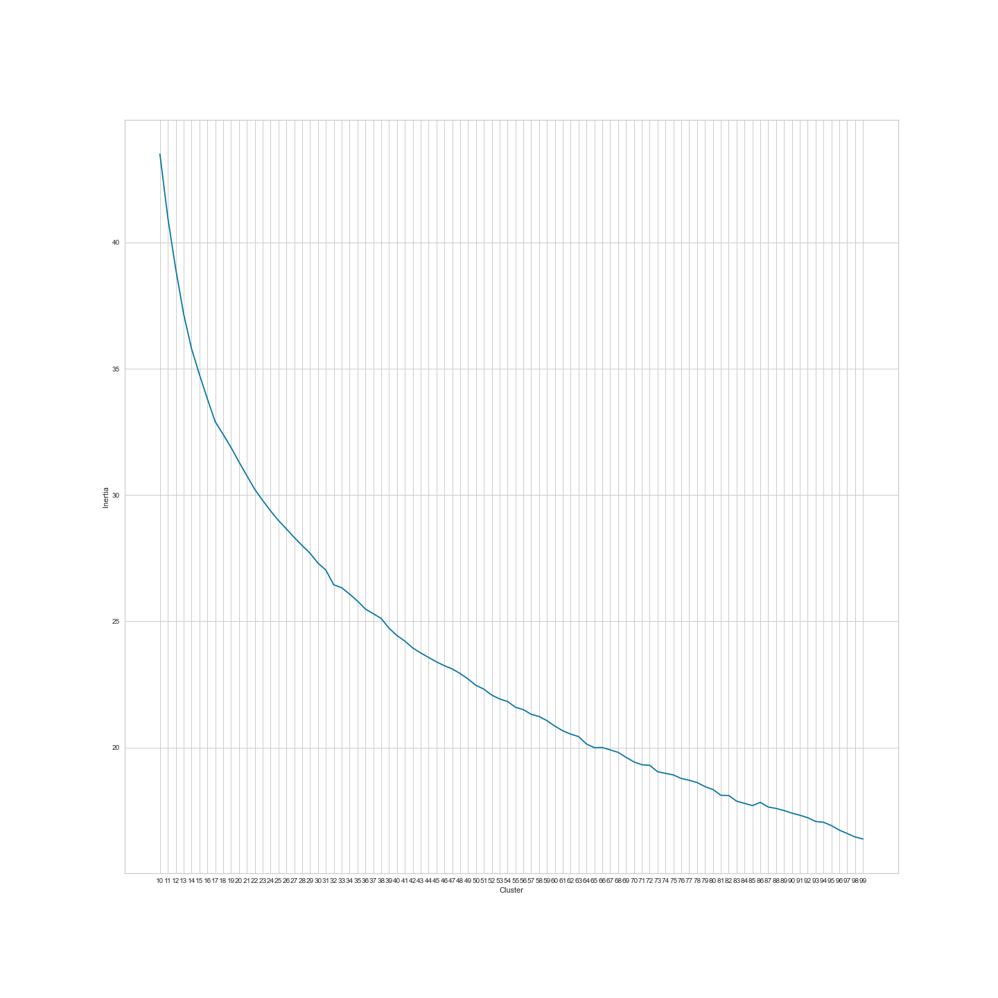
Figure 10: Elbow plot with 3 to 99 clusters.
As we can see, there is no real elbow in our plot this time. This might imply that there are no big clusters in our RELIGION_abstracts.csv dataset. But is it likely that a journal such as Religion that covers a vast spectrum of phenomena (which are all, of course, related to religion) only comprises a few thematic clusters? Probably not. Therefore, let us continue by skipping the silhouette score plots (which are most likely of no value with such a huge number of clusters) and just train a k-means instance with n=100 clusters and assess the results.
kmeans = KMeans(n_clusters=100, random_state=42)
abstracts_labels = kmeans.fit_predict(df_abstracts_pca)
df_abstracts_labeled = df_abstracts.copy()
df_abstracts_labeled["cluster"] = abstracts_labels
We will next evaluate the results by printing out some article titles of randomly chosen clusters. For instance, when analyzing the titles in cluster 75, we can perceive that all articles in this cluster are related to Theravāda Buddhism, Karma, and their perception in “the West”:
df_abstracts_labeled[df_abstracts_labeled["cluster"] == 75][["title", "cluster"]]
| title | cluster | |
|---|---|---|
| 210 | Checking the heavenly ‘bank account of karma’: cognitive metaphors for karma in Western perception and early Theravāda Buddhism | 75 |
| 211 | Karma accounts: supplementary thoughts on Theravāda, Madhyamaka, theosophy, and Protestant Buddhism | 75 |
| 258 | Resonant paradigms in the study of religions and the emergence of Theravāda Buddhism | 75 |
Cluster 15 includes articles related to the body and its destruction:
df_abstracts_labeled[df_abstracts_labeled["cluster"] == 15][["title", "cluster"]]
| title | cluster | |
|---|---|---|
| 361 | Candanbālā’s hair: Fasting, beauty, and the materialization of Jain wives | 15 |
| 425 | Monkey kings make havoc: Iconoclasm and murder in the Chinese cultural revolution | 15 |
| 623 | Techniques of body and desire in Kashmir Śaivism | 15 |
| 695 | Body-symbols and social reality: Resurrection, incarnation and asceticism in early Christianity | 15 |
To be fair, other clusters are harder to interpret. A good example is cluster 84. Yet, even in the case of cluster 84 there still seems to be a pattern, namely that almost all articles are related to famous scholars and works in the study of religion, such as Durkheim, Tylor, Otto, Said, etc.
df_abstracts_labeled[df_abstracts_labeled["cluster"] == 84][["title", "cluster"]]
| title | cluster | |
|---|---|---|
| 80 | Latin America 1520–1600: a page in the history of the study of religion | 84 |
| 141 | On elves and freethinkers: criticism of religion and the emergence of the literary fantastic in Nordic literature | 84 |
| 262 | Is Durkheim’s understanding of religion compatible with believing? | 84 |
| 302 | Dreaming and god concepts | 84 |
| 426 | Orientalism, representation and religion: The reality behind the myth | 84 |
| 448 | The Science of Religions in a Fascist State: Rudolf Otto and Jakob Wilhelm Hauer During the Third Reich | 84 |
| 458 | Religion Within the Limits of History: Schleiermacher and Religion—A Reappraisal | 84 |
| 570 | Cognitive and Ideological Aspects of Divine Anthropomorphism | 84 |
| 571 | Tylor’s Anthropomorphic Theory of Religion | 84 |
| 614 | ‘All my relatives’: Persons in Oglala religion | 84 |
| 650 | Colloquium: Does autonomy entail theology? Autonomy, legitimacy, and the study of religion | 84 |
As we can see, even a simple implementation of k-means on textual data without much feature-tuning has resulted in a k-means instance that is, despite its shortcomings, able to assist us by doing the work of a basic recommender system. For example, we could use our trained k-means instance to suggest articles to visitors of our website based on their previous readings. Of course, we can also use our model during our exploratory data analysis to show us thematic clusters discussed in Religion.
Yet, as the textual data in this example is rather difficult to cluster and includes noise points or clusters that contain very few articles, it might make better sense to apply a different clustering algorithm and see how it performs.
5. Applying DBSCAN Clustering on Textual Data
Even though the k-means clustering of our data already resulted in some valuable insights, it might still be interesting to apply a different clustering algorithm such as DBSCAN. As explained above, DBSCAN excludes noise points and outliers in our data, meaning that it focuses on those regions in our data that may rightfully be called dense.
We will be using the d=10 reduced version of our RELIGION_abstracts.csv dataset, which allows us to use Euclidean distance as a metric. If we were to use the initial TF-IDF matrix with 250 features, we would need to consider changing the underlying metric to cosine distance, which is more suitable when dealing with sparse matrices, as in the case of textual data.
The first step will be to use our findOptimalEps() function to figure out which eps value is most suitable for our data.
findOptimalEps(2, df_abstracts_tfidf)
As can be seen in figure 11, the eps-plotting suggests choosing an eps value between 0.2 and 0.25.
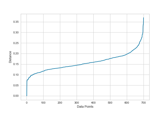
Figure 11: Eps plot for the abstracts dataset.
We are selecting 0.2 as eps value and train a DBSCAN instance.
dbscan = DBSCAN(eps=0.2, metric="euclidean")
dbscan_labels = dbscan.fit_predict(df_abstracts_pca)
df_abstracts_dbscan = df_abstracts.copy()
df_abstracts_dbscan["cluster"] = dbscan_labels
df_abstracts_dbscan["cluster"].unique()
As we can see when looking at the DBSCAN results in our Jupyter notebook, using a DBSCAN instance under these circumstances results in only four clusters and a vast noise points cluster (-1) with more than 150 entries and an even bigger cluster with more than 500 entries (cluster 0). These clusters are plotted in figure 12 (using a PCA-reduced dataset), where the inconclusive results become even more visible. In this case, we could consider using the original TF-IDF matrix with cosine distance instead.
Its shortcomings aside, the current version of our DBSCAN instance does give some promising insights, for example with cluster 3, which collects articles related to gender and women in different religions:
df_abstracts_dbscan[df_abstracts_dbscan["cluster"] == 1][["title", "cluster"]]
| title | cluster | |
|---|---|---|
| 154 | Lifelong minority religion: routines and reflexivity: A Bourdieuan perspective on the habitus of elderly Finnish Orthodox Christian women | 1 |
| 161 | Quiet beauty: problems of agency and appearance in evangelical Christianity | 1 |
| 388 | Renunciation feminised? Joint renunciation of female–male pairs in Bengali Vaishnavism | 1 |
| 398 | Conclusion: Construction sites at the juncture of religion and gender | 1 |
| 502 | Gender and the Contest over the Indian Past | 1 |
| 506 | Art as Neglected ‘Text’ for the Study of Gender and Religion in Africa | 1 |
| 507 | A Medieval Feminist Critique of the Chinese World Order: The Case of Wu Zhao (r. 690–705) | 1 |
| 509 | Notions of Destiny in Women’s Self-Construction | 1 |
| 526 | The Fundamental Unity of the Conservative and Revolutionary Tendencies in Venezuelan Evangelicalism: The Case of Conjugal Relations | 1 |
| 551 | Hindu Women, Destiny and Stridharma | 1 |
| 644 | The women around James Nayler, Quaker: A matter of emphasis | 1 |
| 668 | Women as aspects of the mother Goddess in India: A case study of Ramakrishna | 1 |
Cluster 2, on the other hand, seems to be related to belief and atheism:
df_abstracts_dbscan[df_abstracts_dbscan["cluster"] == 2][["title", "cluster"]]
| title | cluster | |
|---|---|---|
| 209 | Three cognitive routes to atheism: a dual-process account | 2 |
| 282 | THE CULTURAL TRANSMISSION OF FAITH Why innate intuitions are necessary, but insufficient, to explain religious belief | 2 |
| 321 | Religion is natural, atheism is not: On why everybody is both right and wrong | 2 |
| 322 | Atheism is only skin deep: Geertz and Markusson rely mistakenly on sociodemographic data as meaningful indicators of underlying cognition | 2 |
| 323 | The relative unnaturalness of atheism: On why Geertz and Markússon are both right and wrong | 2 |
| 378 | The science of religious beliefs | 2 |
| 380 | Adaptation, evolution, and religion | 2 |
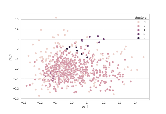
Figure 12: PCA-reduced version of the abstracts dataset displaying the DBSCAN clustering with eps=0.2.
Although the clustering was far from perfect in this case, it did produce some valuable information, which we could use in combination with the more promising results of the k-means clustering. It might also be pertinent to keep tuning the parameters and trying out different feature sets (reduced, non-reduced, maybe by adding some additional feature selection steps of choosing promising word fields, etc.) to achieve better results with DBSCAN. Of course, we could also apply some other clustering algorithms and then combine the results.
As a next step, we could pursue the idea of building a basic recommender system which suggests articles with similar topics to readers based on their previous readings. This recommender system should consider the clustering of the k-means instance but also include suggestions made by DBSCAN and other potential clustering algorithms. When applied in combination, the rather unsatisfactory results of the DBSCAN model might be less problematic because they are now used as additional information only.
Of course, we as scholars in the humanities will be more likely to use these techniques as part of our research during the exploratory data analysis phase. In this case, combining the results of different clustering algorithms helps us to discover structures and thematic clusters in our data. These discoveries could then lead to new research questions. For instance, there might be specific clusters in the Religion abstracts data that include more articles than the other clusters, thereby indicating an overall thematic focus of this journal that might be worth examining to get an overview of research trends in the study of religion throughout recent decades.
Summary
I hope to have shown that clustering is indeed a valuable step during exploratory data analysis that enables you to gain new insights into your data.
The clustering of the DNP_ancient_authors.csv and the RELIGION_abstracts.csv datasets provided decent results and identified reasonable groupings of authors and articles in the data. In the case of the abstracts dataset, we have even built a basic recommender system that assists us when searching for articles with similar topics. Yet, the discussion of the results also illustrated that there is always room for interpretation and that not every cluster necessarily needs to provide useful insights from a scholarly (or human) perspective. Despite this general ambiguity when applying machine learning algorithms, our analysis demonstrated that k-means and DBSCAN are great tools that can help you to develop or empirically support new research questions. In addition, they may also be implemented for more practical tasks, for instance, when searching for articles related to a specific topic.
Bibliography
- Géron, Aurélien. Hands-on machine learning with Scikit-Learn, Keras, and TensorFlow. Concepts, tools, and techniques to build intelligent systems, 2nd ed. Sebastopol: O’Reilly, 2019.
- Mitchell, Ryan. Web scraping with Python. Collecting more data from the modern web, 1st ed. Sebastopol: O’Reilly, 2018.
- Patel, Ankur A. Hands-on unsupervised learning using Python: How to build applied machine learning solutions from unlabeled data, 1st ed. Sebastopol: O’Reilly, 2019.
Footnotes
-
For a good introduction to the use of requests and web scraping in general, see the corresponding articles on The Programming Historian such as Introduction to BeautifulSoup (last accessed: 2021-04-22) or books such as Mitchell (2018). ↩
-
Yet, there are certain cases where k-means clustering might fail to identify the clusters in your data. Thus, it is usually recommended to apply several clustering algorithms. A good illustration of the restrictions of k-means clustering can be seen in the examples under this link (last accessed: 2021-04-23) to the scikit-learn website, particularly in the second plot on the first row. ↩
-
Definition of inertia on scikit-learn (last accessed: 2021-04-23). ↩