Lesson Goals
This lesson explains why many cultural institutions are adopting graph databases, and how researchers can access these data though the query language called SPARQL.
Contents
- Lesson Goals
- Graph Databases, RDF, and Linked Open Data
- Real-world queries
- Working with SPARQL results
- Further reading
Graph Databases, RDF, and Linked Open Data
Many cultural institutions now offer access to their collections information through web Application Programming Interfaces. While these APIs are a powerful way to access individual records in a machine-readable manner, they are not ideal for cultural heritage data because they are structured to work for a predetermined set of queries. For example, a museum may have information on donors, artists, artworks, exhibitions, and provenance, but its web API may offer only object-wise retrieval, making it difficult or impossible to search for associated data about donors, artists, provenance, etc. This structure is great if you come looking for information about particular objects. However, it makes it difficult to aggregate information about every artist or donor that happens to be described in the dataset as well.
RDF databases are well-suited to expressing complex relationships between many entities, like people, places, events, and concepts tied to individual objects. These databases are often referred to as “graph” databases because they structure information as a graph or network, where a set of resources, or nodes, are connected together by edges that describe the relationships between each resource.
Because RDF databases support the use of URLs (weblinks), they can be made available online and linked to other databases, hence the term “Linked Open Data”. Major art collections including the British Museum, Europeana, the Smithsonian American Art Museum, and the Yale Center for British Art have published their collections data as LOD. The Getty Vocabulary Program, has also released their series of authoritative databases on geographic place names, terms for describing art and architecture, and variant spellings of artist names, as LOD.
SPARQL is the language used to query these databases. This language is particularly powerful because it does not presuppose the perspectives that users will bring to the data. A query about objects and a query about donors is basically equivalent to such a database. Unfortunately, many tutorials on SPARQL use extremely simplified data models that don’t resemble the more complex datasets released by cultural heritage institutions. This tutorial gives a crash course on SPARQL using a dataset that a humanist might actually find in the wilds of the Internet. In this tutorial, we will learn how to query the British Museum Linked Open Data collection.
RDF in brief
RDF represents information in a series of three-part “statements” that comprise a subject, predicate, and an object, e.g.:
<The Nightwatch> <was created by> <Rembrandt van Rijn> .
(Note that just like any good sentence, they each have a period at the end.)
Here, the subject <The Nightwatch> and the object <Rembrandt van Rijn> can
be thought of as two nodes of the graph, with the predicate <was created by>
defining an edge between them. (Technically, <was created by> can, in other
queries, be treated as an object or subject itself, but that is beyond the scope
of this tutorial.)
A pseudo-RDF database might contain interrelated statements like these:
...
<The Nightwatch> <was created by> <Rembrandt van Rijn> .
<The Nightwatch> <was created in> <1642> .
<The Nightwatch> <has medium> <oil on canvas> .
<Rembrandt van Rijn> <was born in> <1606> .
<Rembrandt van Rijn> <has nationality> <Dutch> .
<Johannes Vermeer> <has nationality> <Dutch> .
<Woman with a Balance> <was created by> <Johannes Vermeer> .
<Woman with a Balance> <has medium> <oil on canvas> .
...
If we were to visualize these statements as nodes and edges within network graph, it would appear like so:

A network visualization of the pseudo-RDF shown above. Arrows indicate the ‘direction’ of the predicate. For example, that ‘Woman with a Balance was created by Vermeer’, and not the other way around.
A traditional relational database might split attributes about artworks and attributes about artists into separate tables. In an RDF/graph database, all these data points belong to the same interconnected graph, which allows users maximum flexibility in deciding how they wish to query it.
Searching RDF with SPARQL
SPARQL lets us translate heavily interlinked, graph data into normalized, tabular data with rows and columns you can open in programs like Excel, or import into a visualization suite such as plot.ly or Palladio.
It is useful to think of a SPARQL query as a Mad Lib - a set of sentences with blanks in them. The database will take this query and find every set of matching statements that correctly fill in those blanks, returning the matching values to us as a table. Take this SPARQL query:
SELECT ?painting
WHERE {
  ?painting <has medium> <oil on canvas> .
}
?painting in this query stands in for the node (or nodes) that the database
will return. On receiving this query, the database will search for all values of
?painting that properly complete the RDF statement <has medium> <oil on
canvas> .:

A visualization of what our query is looking for.
When the query runs against the full database, it looks for the subjects, predicates, and objects that match this statement, while excluding the rest of the data:

A visualization of the SPARQL query, with mentioned elements in orange, and selected elements (those that will be returned in the results) in red.
And our results might look like this table:
| painting |
|---|
| The Nightwatch |
| Woman with a Balance |
What makes RDF and SPARQL powerful is the ability to create complex queries that reference many variables at a time. For example, we could search our pseudo-RDF database for paintings by any artist who is Dutch:
SELECT ?artist ?painting
WHERE {
  ?artist <has nationality> <Dutch> .
  ?painting <was created by> ?artist .
}
Here we’ve introduced a second variable, ?artist. The RDF database will return
all matching combinations of ?artist and ?painting that fulfill both of
these statements.

A visualization of the SPARQL query, with mentioned elements in orange, and selected elements (those that will be returned in the results) in red.
| artist | painting |
|---|---|
| Rembrandt van Rijn | The Nightwatch |
| Johannes Vermeer | Woman with a Balance |
URIs and Literals
So far, we have been looking at a toy representation of RDF that uses easy-to-read text. However, RDF is primarily stored as URIs (Uniform Resource Identifiers) that separate conceptual entities from their plain-English (or other language!) labels. (Note that a URL, or Uniform Resource Locator, is a URI for a resource that is accessible on the web) In real RDF, our original statement:
<The Nightwatch> <was created by> <Rembrandt van Rijn> .
would more likely look something like this:
<http://data.rijksmuseum.nl/item/8909812347> <http://purl.org/dc/terms/creator> <http://dbpedia.org/resource/Rembrandt>.
N.B. the Rijksmuseum has not (yet) built their own Linked Data site, so the URI in this query is just for demo purposes.
In order to get the human-readable version of the information represented by each of these URIs, what we’re really doing is just retrieving more RDF statements. Even the predicate in that statement has its own literal label:
<http://data.rijksmuseum.nl/item/8909812347> <http://purl.org/dc/terms/title> "The Nightwatch" .

<http://purl.org/dc/terms/creator> <http://www.w3.org/1999/02/22-rdf-syntax-ns#label> "was created by" .

<http://dbpedia.org/resource/Rembrandt> <http://xmlns.com/foaf/0.1/name> "Rembrandt van Rijn" .
You will notice that, unlike the URIs in the query that are surrounded by <>,
the objects of these statements are just strings of text within quotation
marks, known as literals. Literals are unlike URIs in that they represent
values, rather than references. For example,
<http://dbpedia.org/resource/Rembrandt> represents an entity that may
reference (and be referenced by) any number of other statements (say, birth
dates, students, or family members), while the text string "Rembrandt van
Rijn" stands only for itself. Literals do not point to other nodes in the
graph, and they can only ever be objects in an RDF statement. Other literal
values in RDF include dates and numbers.
See the predicates in these statements, with domain names like purl.org,
w3.org, and xmlns.com? These are some of the many providers of ontologies
that help standardize the way we describe relationships between bits of
information like “title”, “label”, “creator”, or “name”. The more RDF/LOD that
you work with, the more of these providers you’ll find.
URIs can become unwieldy when composing SPARQL queries, which is why we’ll
use prefixes. These are shortcuts that allow us to skip typing out entire long
URIs. For example, remember that predicate for retrieving the title of the
Nightwatch, <http://purl.org/dc/terms/title>? With these prefixes, we just
need to type dct:title whenever we need to use a purl.org predicate. dct:
stands in for http://purl.org/dc/terms/, and title just gets pasted onto the
end of this link.
For example, with the prefix PREFIX rkm: <http://data.rijksmuseum.nl/>,
appended to the start of our SPARQL query,
<http://data.rijksmuseum.nl/item/8909812347> becomes rkm:item/8909812347
instead.
Be aware that, prefixes
can be arbitrarily assigned with whatever abbreviations you like, different
endpoints may use slightly different prefixes for the same namespace (e.g. dct
vs. dcterms for <http://purl.org/dc/terms/>).
Terms to review
- SPARQL - Protocol and RDF Query Language - The language used to query RDF graph databases
- RDF - Resource Description Framework - A method for structuring data as a graph or network of connected statements, rather than a series of tables.
- LOD - Linked Open Data - LOD is RDF data published online with dedicated URIs in such a manner than developers can reliably reference it.
- statement - Sometimes also called a “triple”, an RDF statement is a quantum of knowledge comprising a subject, predicate, and object.
- URI - Uniform Resource Identifier - a string of characters for identifying a resource. RDF statements use URIs to link various resources together. A URL, or uniform resource locator, is a type of URI that points to resources on the web.
- literal - Some objects in RDF statements do not refer to other resources with a URI, but instead convey a value, such as text (
"Rembrandt van Rijn"), a number (5), or a date (1606-06-15). These are known as literals. - prefix - In order to simplify SPARQL queries, a user may specify prefixes that act as abbreviations for full URIs. These abbreviations, or QNames, are also used in namespaced XML documents.
Real-world queries
All the statements for one object
Let’s start our first query using the British Museum SPARQL endpoint. A SPARQL endpoint is a web address that accepts SPARQL queries and returns results. The BM endpoint is like many others: if you navigate to it in a web browser, it presents you with a text box for composing queries.
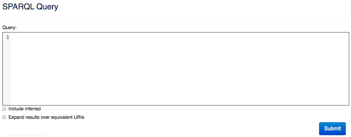
The BM SPARQL endpoint webpage. For all the queries in this tutorial, make sure that you have left the ‘Include inferred’ and ‘Expand results over equivalent URIs’ boxes unchecked.
When starting to explore a new RDF database, it helps to look at the relationships that stem from a single example object.
(For each of the following queries, click on the “Run query” link below to see the results. You can then run it as is, or modify it before requesting the results. Remember when editing the query before running to uncheck the ‘Include inferred’ box.)
SELECT ?p ?o
WHERE {
  <http://collection.britishmuseum.org/id/object/PPA82633> ?p ?o .
}
By calling SELECT ?p ?o we’re asking the database to return the values of ?p
and ?o as described in the WHERE {} command. This query returns every
statement for which our example artwork,
<http://collection.britishmuseum.org/id/object/PPA82633>, is the subject. ?p
is in the middle position of the RDF statement in the WHERE {} command, so it
returns any predicates matching this statement, while ?o in the final position
returns all objects. Though I have named them ?p and ?o here, as you will
see below we can name these variables anything we like. Indeed, it will be
useful to give them meaningful names for the complex queries that follow!.
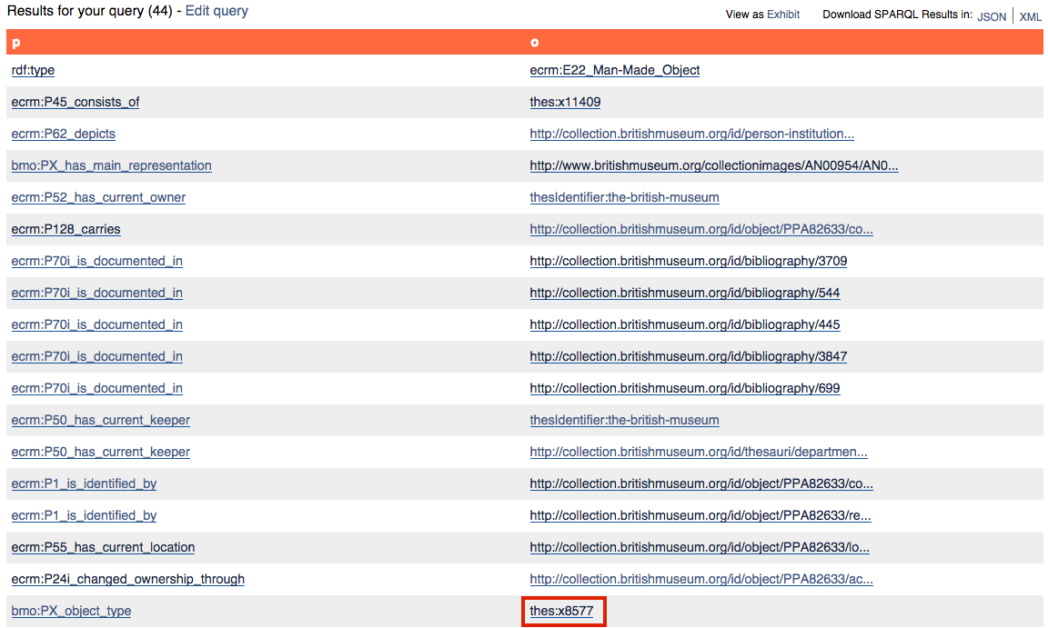
An initial list of all the predicates and objects associated with one artwork in the British Museum.
Note: depending on how the British Museum has configured their SPARQL endpoint when you read this lesson, instead of seeing “prefixed” versions of the URLs (e.g. thes:8577) you may instead see the full version http://collection.britishmuseum.org/id/thesauri/x8577. As noted in the discussion of prefixes above, this still represents the same URI.
The BM endpoint formats the results table with hyperlinks for every variable that is itself an RDF node, so by clicking on any one of these links you can shift to seeing all the predicates and objects for that newly-selected node. Note that BM automatically includes a wide range of SPARQL prefixes in its queries, so you will find many hyperlinks are displayed in their abbreviated versions; if you mouse over them your browser will display their unabbreviated URIs.

Visualizing a handful of the nodes returned by the first query to the BM. Elements in this graph that are also in the table of results above are colored red. Additional levels in the hierarchy are included as a preview of how this single print connects to the larger BM graph.
Let’s find out how they store the object type information: look for the
predicate <bmo:PX_object_type> (highlighted in the figure above) and click on
the link for thes:x8577 to navigate to the node describing the particular
object type “print”:
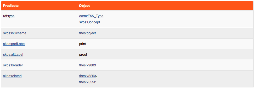
The resource page for thes:x8577 (‘print’) in the British Museum LOD.
You’ll note how this node has an plain-text label, as well as ties to related artwork type nodes within the database.
Complex queries
To find other objects of the same type with the preferred label “print”, we can call this query:
PREFIX bmo: <http://www.researchspace.org/ontology/>
PREFIX skos: <http://www.w3.org/2004/02/skos/core#>

SELECT ?object
WHERE {

  # Search for all values of ?object that have a given "object type"
  ?object bmo:PX_object_type ?object_type .

  # That object type should have the label "print"
  ?object_type skos:prefLabel "print" .
}
LIMIT 10
Run query / See a user-generated query
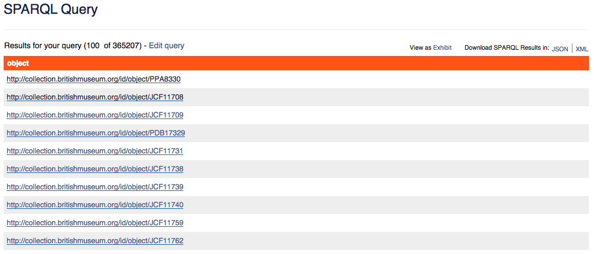
A one-column table returned by our query for every object with type ‘print’
Remember that, because "print" here is a literal, we enclose it within
quotation marks in our query. When you include literals in a SPARQL query, the
database will only return exact matches for those values.
Note that, because ?object_type is not present in the SELECT command, it
will not show up in the results table. However, it is essential to structuring
our query, because it connects the dots from ?object to the label "print".
FILTER
In the previous query, our SPARQL query searched for an exact match for the
object type with the text label “print”. However, often we want to match literal
values that fall within a certain range, such as dates. For this, we’ll use the
FILTER command.
To find URIs for all the prints in the BM created between 1580 and 1600, we’ll need to first figure out where the database stores dates in relationship to the object node, and then add references to those dates in our query. Similar to the way that we followed a single link to determine an object type, we must hop through several nodes to find the production dates associated with a given object:

Visualizing part of the British Museum’s data model where production dates are connected to objects.
PREFIX bmo: <http://www.researchspace.org/ontology/>
PREFIX skos: <http://www.w3.org/2004/02/skos/core#>
PREFIX ecrm: <http://www.cidoc-crm.org/cidoc-crm/>
PREFIX xsd: <http://www.w3.org/2001/XMLSchema#>

# Return object links and creation date
SELECT ?object ?date
WHERE {

  # We'll use our previous command to search only for
  # objects of type "print"
  ?object bmo:PX_object_type ?object_type .
  ?object_type skos:prefLabel "print" .

  # We need to link though several nodes to find the
  # creation date associated with an object
  ?object ecrm:P108i_was_produced_by ?production .
  ?production ecrm:P9_consists_of ?date_node .
  ?date_node ecrm:P4_has_time-span ?timespan .
  ?timespan ecrm:P82a_begin_of_the_begin ?date .

  # As you can see, we need to connect quite a few dots
  # to get to the date node! Now that we have it, we can
  # filter our results. Because we are filtering by date,
  # we must attach the tag ^^xsd:date after our date strings.
  # This tag tells the database to interpret the string
  # "1580-01-01" as the date 1 January 1580.

  FILTER(?date >= "1580-01-01"^^xsd:date &&
         ?date <= "1600-01-01"^^xsd:date)
}

All BM prints made between 1580 and 1600
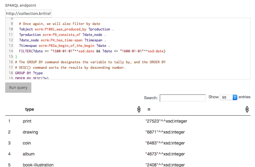
Aggregation
So far we have only used the SELECT command to return a table of objects.
However, SPARQL allows us to do more advanced analysis such as grouping,
counting, and sorting.
Say we would like to keep looking at objects made between 1580 and 1600, but we
want to understand how many objects of each type the BM has in its collections.
Instead of limiting our results to objects of type “print”, we will instead use
COUNT to tally our search results by type.
PREFIX bmo: <http://www.researchspace.org/ontology/>
PREFIX skos: <http://www.w3.org/2004/02/skos/core#>
PREFIX ecrm: <http://www.cidoc-crm.org/cidoc-crm/>
PREFIX xsd: <http://www.w3.org/2001/XMLSchema#>

SELECT ?type (COUNT(?type) as ?n)
WHERE {
  # We still need to indicate the ?object_type variable,
  # however we will not require it to match "print" this time

  ?object bmo:PX_object_type ?object_type .
  ?object_type skos:prefLabel ?type .

  # Once again, we will also filter by date
  ?object ecrm:P108i_was_produced_by ?production .
  ?production ecrm:P9_consists_of ?date_node .
  ?date_node ecrm:P4_has_time-span ?timespan .
  ?timespan ecrm:P82a_begin_of_the_begin ?date .
  FILTER(?date >= "1580-01-01"^^xsd:date &&
         ?date <= "1600-01-01"^^xsd:date)
}
# The GROUP BY command designates the variable to tally by,
# and the ORDER BY DESC() command sorts the results by
# descending number.
GROUP BY ?type
ORDER BY DESC(?n)
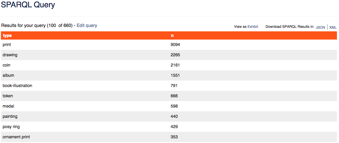
Counts of objects by type produced between 1580 and 1600.
Linking multiple SPARQL endpoints
Up until now, we have constructed queries that look for patterns in one dataset alone. In the ideal world envisioned by Linked Open Data advocates, multiple databases can be interlinked to allow very complex queries dependent on knowledge present in different locations. However, this is easier said than done, and many endpoints (the BM’s included) do not yet reference outside authorities.
One endpoint that does, however, is
Europeana’s. They have created links
between the objects in their database and records about individuals in
DBPedia and VIAF, places in
GeoNames, and concepts in the Getty Art &
Architecture thesaurus. SPARQL allows you to insert SERVICE statements that
instruct the database to “phone a friend” and run a portion of the query on
an outside dataset, using the results to complete the query on the local
dataset. While this lesson will go into the data models in Europeana and DBpedia in depth, the following query illustrates how a SELECT statement works. You may run it yourself by copying and pasting the query text into the Europeana endpoint.
PREFIX edm:    <http://www.europeana.eu/schemas/edm/>
PREFIX rdf:    <http://www.w3.org/1999/02/22-rdf-syntax-ns#>
PREFIX dbo:    <http://dbpedia.org/ontology/>
PREFIX dbr:    <http://dbpedia.org/resource/>
PREFIX rdaGr2: <http://rdvocab.info/ElementsGr2/>

# Find all ?object related by some ?property to an ?agent born in a
# ?dutch_city
SELECT ?object ?property ?agent ?dutch_city
WHERE {
    ?proxy ?property ?agent .
    ?proxy ore:proxyFor ?object .

    ?agent rdf:type edm:Agent .
    ?agent rdaGr2:placeOfBirth ?dutch_city .

    # ?dutch_city is defined by having "Netherlands" as its broader
    # country in DBpedia. The SERVICE statement asks
    # http://dbpdeia.org/sparql which cities have the country
    # "Netherlands". The answers to that sub-query will then be
    # used to finish off our original query about objects in the
    # Europeana database

    SERVICE <http://dbpedia.org/sparql> {
        ?dutch_city dbo:country dbr:Netherlands .
   }
}
# This query can potentially return a lot of objects, so let's
# just request the first 100 in order to speed up the search
LIMIT 100
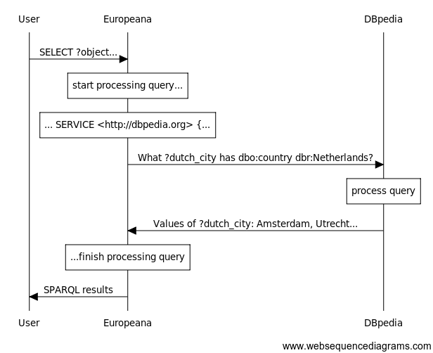
Visualizing the query sequence of the above SPARQL request
An interlinked query like this means that we can ask Europeana questions about its objects that rely on information about geography (what cities are in the Netherlands?) that Europeana does not need to store and maintain itself. In the future, more cultural LOD will hopefully link to authority databases like the Getty’s Union List of Artist Names, allowing, for example, the British Museum to outsource biographical data to the more complete resources at the Getty.
Working with SPARQL results
Having constructed and run a query… what do we do with the results? Many endpoints offer, like the British Museum, a web-based browser that returns human-readable results. However, SPARQL endpoints are designed to return structured data to be used by other programs.
Export results to CSV
In the top right corner of the results page for the BM endpoint, you will find
links for both JSON and XML downloads. Other endpoints may also offer the
option for a CSV/TSV download, however this option is not always available. The
JSON and XML output from a SPARQL endpoint contain not only the values returned
from the SELECT statement, but also additional metadata about variable types
and languages.
Parsing the XML verson of this output may be done with a tool like Beautiful Soup (see its Programming Historian lesson) or Open Refine. To quickly convert JSON results from a SPARQL endpoint into a tabular format, I recommend the free command line utility jq. (For a tutorial on using command line programs, see “Introduction to the Bash Command Line”.) The following query will convert the special JSON RDF format into a CSV file, which you may load into your preferred program for further analysis and visualization:
jq -r '.head.vars as $fields | ($fields | @csv), (.results.bindings[] | [.[$fields[]].value] | @csv)' sparql.json > sparql.csv
Export results to Palladio
The popular data exploration platform Palladio can directly load data from a
SPARQL endpoint. On the “Create a new project” screen, a link at the bottom to
“Load data from a SPARQL endpoint (beta)” will provide you a field to enter the
endpoint address, and a box for the query itself. Depending on the endpoint, you
may need to specify the file output type in the endpoint address; for example,
to load data from the BM endpoint you must use the address
http://collection.britishmuseum.org/sparql.json. Try pasting in the
aggregation query we used above to count artworks by type and clicking on “Run
query”. Palladio should display a preview table.
Palladio’s SPARQL query interface.
After previewing the data returned by the endpoint, click on the “Load data” button at the bottom of the screen to begin manipulating it. (See this Programming Historian lesson for a more in-depth tutorial on Palladio.) For example, we might make a query that returns links to the images of prints made between 1580 and 1600, and render that data as a grid of images sorted by date:
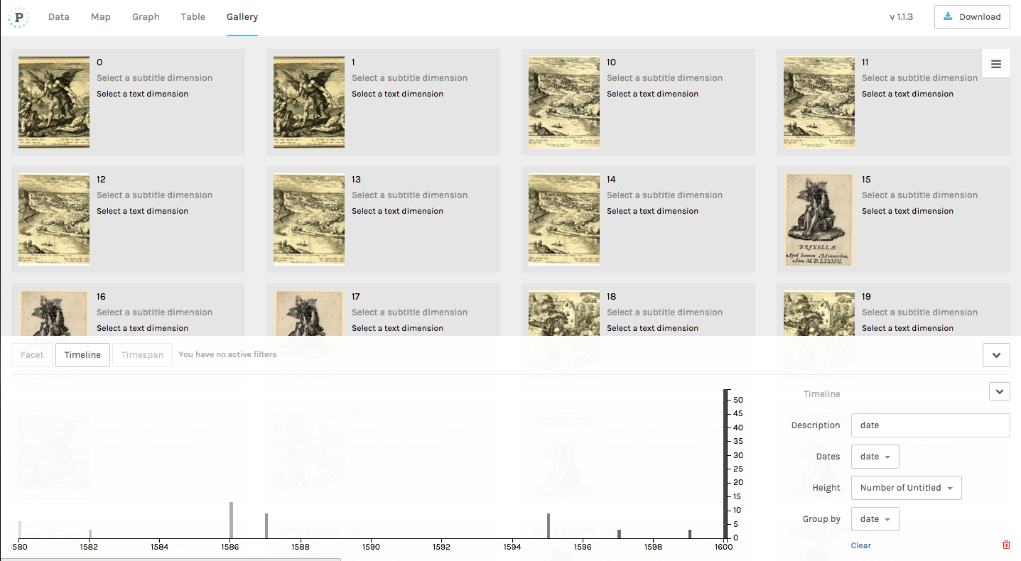
A gallery of images with a timeline of their creation dates generated using Palladio.
Note that Palladio is designed to work with relatively small amounts of data (on
the order of hundreds or thousands of rows, not tens of thousands), so you may
have to use the LIMIT command that we used when querying the Europeana
endpoint to reduce the number of results that you get back, just to keep the
software from freezing.
Further reading
In this tutorial we got a look at the structure of LOD as well as a real-life example of how to write SPARQL queries for the British Museum’s database. You also learned how to use aggregation commands in SPARQL to group, count, and sort results rather than simply list them.
There are even more ways to modify these queries, such as introducing OR and
UNION statements (for describing conditional queries), and CONSTRUCT
statements (for inferring new links based on defined rules), full-text
searching, or doing other mathematical operations more complex than counting.
For a more complete rundown of the commands available in SPARQL, see these
links:
Both the Europeana and Getty Vocabularies LOD sites also offer extensive, and quite complex example queries which can be good sources for understanding how to search their data:
