
Contents
- Introduction
- Preparation
- OCR with Tesseract
- OCR with Google Vision
- Combining Layout and Character Recognition
- Conclusions
Introduction
Historians working with digital methods and text-based material are often confronted with PDF files that need to be converted to plain text. Whether you are interested in network analysis, named entity recognition, corpus linguistics, text reuse, or any other type of text-based analysis, good quality Optical Character Recognition (OCR), which transforms a PDF to a computer-readable file, will be the first step. However, OCR becomes trickier when dealing with historical fonts and characters, damaged manuscripts or low-quality scans. Fortunately, tools such as Tesseract, TRANSKRIBUS, OCR4all, eScriptorium and OCR-D (among others) have allowed humanities scholars to work with all kinds of documents, from handwritten nineteenth-century letters to medieval manuscripts.
Despite these great tools, it can still be difficult to find an OCR solution that aligns with our technical knowledge, can be easily integrated within a workflow, or can be applied to a multilingual/diverse corpus without requiring any extra input from the user. This lesson offers a possible alternative by introducing two ways of combining Google Vision’s character recognition with Tesseract’s layout detection. Google Cloud Vision is one of the best ‘out-of-the-box’ tools when it comes to recognising individual characters but, contrary to Tesseract, it has poor layout recognition capabilities. Combining both tools creates a “one-size-fits-most” method that will generate high-quality OCR outputs for a wide range of documents.
The principle of exploring different combinations of tools to create customised workflows is widely applicable in digital humanities projects, where tools tailored to our data are not always available.
The Pros and Cons of Google Vision, Tesseract, and their Powers Combined
Google Vision
Pros
- Character detection accuracy: Although it has its limitations, Google Vision tends to be highly accurate, even in cases where other tools might struggle, such as when several languages coexist in the same text. It is among the best ‘out-of-the-box’ tools when it comes to recognising characters.
- Versatility: The tool performs well across a wide range of documents. Moreover, Google Vision offers other functionalities such as object detection in images and OCR for handwritten documents/images.
- User-friendliness: Once the setup is completed, Google Vision is easy to use. There is usually no need to develop and train your own model.
- Languages support: At the time of writing, Google Vision fully supports 60 languages. In addition, 36 are under active development and 133 are mapped to another language code or a general character recogniser. Many indigenous, regional, and historical languages are among the latter. You can consult the full list of supported languages in the Cloud Vision documentation.
Cons
- Layout detection accuracy: Although Google Vision performs well with character detection, layout detection is often an issue.
- Google email address and Cloud storage: To sign in to the Google Cloud Platform, a Google email address is required and the PDF files must be uploaded to the Google Cloud Storage to be processed.
- Sustainability: Google Cloud is known for sunsetting tools. Although Google now has a policy in place guaranteeing a year’s notice before deprecating products, the potential instability of the Google Cloud Platform should be noted.
- Cost: The service is only free for the first 1000 pages per month. After that, it costs $1.50 per 1000 pages. Current prices in other currencies are available via Google Cloud Platform services. In addition, to use the OCR functionality of Google Vision, you need to momentarily store your PDF documents in Google Storage. Storing one GB over a month costs $0.02. One GB represents thousands of PDF pages. Since the cost is prorated, if you store 1GB for 12 hours over the course of the month, it will cost $0.0003. Therefore, to avoid paying, you should delete your data from Google Storage as soon as the OCR process is complete. You can find details about the current cost of Google Storage on their pricing page. Although this is not guaranteed, new accounts often come with free credits.
Tesseract
Pros
- Sustainability: Tesseract was originally developed by Hewlett-Packard but was made open scource in 2005. An active community has contributed to its development since. It was also developed by Google from 2006 to 2018.
- Cost: Free.
- Layout detection accuracy: In comparison to Google Vision, Tesseract performs a lot better at layout detection.
- User-friendliness: Contrary to Google Vision, Tesseract does not require any initial setup besides downloading the software. Since it is open source, Tesseract is integrated with many tools and can be used from the command line.
- Languages support: It currently supports over 110 languages including many non-Indo-European languages and writing systems.
Cons
- Character detection accuracy: In comparison to Google Vision, Tesseract does not perform as well with complex characters (for example, historical characters and ligatures).
Combining Google Vision and Tesseract
Tesseract is a great option for clean text for which typography does not present particular challenges. Google Vision will produce high-quality results on more complex characters, as long as the layout is very basic. If your material includes complex characters and layouts (such as columns), the combination of Google Vision and Tesseract will come in handy. This approach takes the best of both worlds —layout recognition from Tesseract and character recognition from Google Vision— and tend to perform better than either method separately.
First Combined Method
The first method for combining the two OCR tools involves building a new PDF from the images of each text region identified by Tesseract. In this new PDF, the text regions are stacked vertically. This means that Google Vision’s inability to identify vertical text separators is no longer a problem.
This method usually performs well, but it still relies on Google Vision for layout detection. Although the vertical stacking of the text regions significantly reduces errors, it is still possible for mistakes to appear, especially if you have many small text regions in your documents. A drawback of this method is that any mapping from the source facsimile/PDF to the resulting text is lost.
Second Combined Method
The second combined method works with the original PDF, but instead of using the OCR text string that Google Vision provides for each page, the JSON output files are searched for the words that fall within the bounds of the text regions identified by Tesseract. This is possible because Google Vision provides coordinates for each word in the document.
This method has the advantage of not relying on Google Vision’s layout detection at all. However, the downside is that line breaks that were not initially identified by Google Vision cannot be easily reintroduced. Therefore, if it is important for your project that the OCRed text retains line breaks at the correct locations, the first combined method will be the best choice.
The following three examples highlight the potential benefits of using Google Vision, Tesseract, or one of the combined methods. Each image represents two pages from the dataset we will be using in this lesson. Outputs created for the passages highlighted in yellow by each of the four methods are detailed in the table below each image.
Comparing Results
Example 1
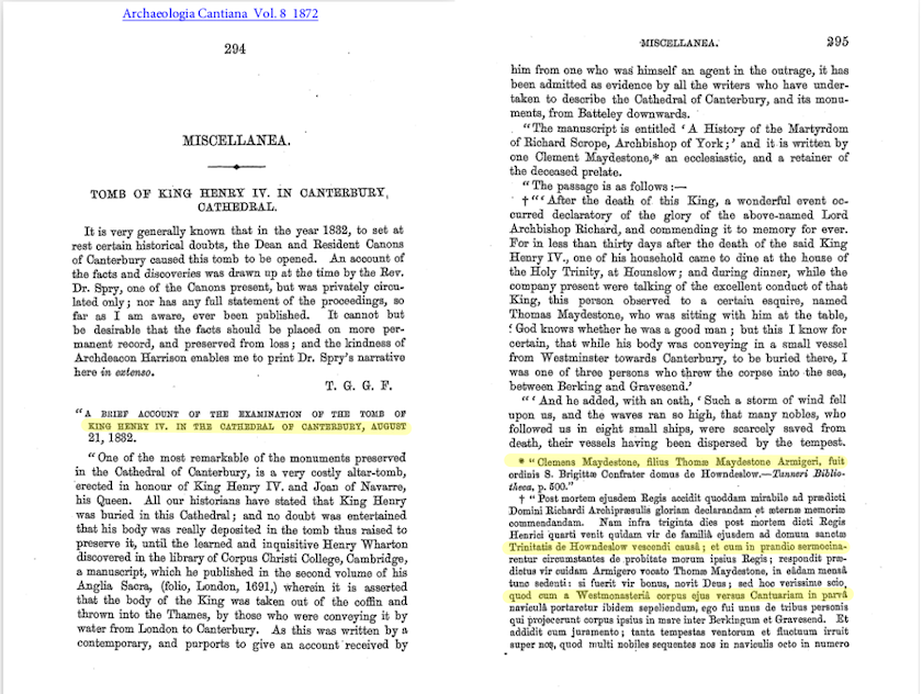
Figure 1: First two pages of Tomb of King Henry IV in Canterbury Cathedral, with four highlighted lines indicating the text used in the OCR results below.
| Google Vision | Tesseract |
|---|---|
| KING BENRY IV. IN THE CATHEDRAL OF CANTERBURY, AUGUST | KING HENRY IV. IN THE CATHEDRAL OF CANTERBURY, AUGUST |
| ** Clemens Maydestone, filius Thomæ Maydestone Armigeri, fuit | * * Olemens Maydestone, filius Thoms Maydestone Armigeri, fuit |
| Trinitatis de Howndeslow. vescendi causâ; et cum in prandio sermocina- | Trinitatis de Howndeslow vescendi eaus&; et cum in prandio sermocina- |
| quod cum a Westmonasteriâ corpus ejus versus Cantuariam in paiva | quod eum a Westmonasterii corpus ejus versus Cantuariam in parva |
| Combined Method I | Combined Method II |
|---|---|
| KING HENRY IV. IN THE CATHEDRAL OF CANTERBURY, AUGUST | KING BENRY IV. IN THE CATHEDRAL OF CANTERBURY, AUGUST |
| * “Clemens Maydestone, filius Thomæ Maydestone Armigeri, fuit | ** Clemens Maydestone, filius Thomæ Maydestone Armigeri, fuit |
| Trinitatis de Howndeslow vescendi causâ ; et cum in prandio sermocina- | Trinitatis de Howndeslow. vescendi causâ ; et cum in prandio sermocina- |
| quod cum a Westmonasteriâ corpus ejus versus Cantuariam in parva | quod cum a Westmonasteriâ corpus ejus versus Cantuariam in paiva |
In the above example, we can observe that words such as “Thomæ” and “causâ” are correctly spelled in all three methods involving Google Vision but are mispelled by Tesseract. The two combined methods perform similarly but the first is the most accurate, notably because of an improved rendering of punctuation.
Example 2
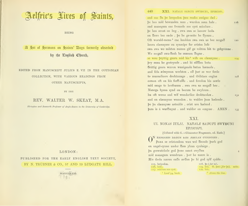
Figure 2: First two pages of Aelfric’s Life of Saints, with several highlighted sections indicating the text used in the OCR results below.
| Google Vision | Tesseract |
|---|---|
| Aelfries Lives of Saints, | Aelfrics Fives of Saints, |
| A Set of Sermons on Saints’ Days formerly observed | A Set of Sermons on Saints’ Days formerly observey |
| BY N. TRÜBNER & CO., 57 AND 59 LUDGATE HILL. | BY N. TRUBNER & CO., 57 AND 59 LUDGATE HILL. |
| XXI. NATALE SANCTI SWYÐUNI, EPISCOPI. | 440 XXI. NATALE SANCTI SWYDUNI, EPISCOPI. |
| and eac da þe hrepodon þæs reafes ænigne dæl. | and eac Sa pe hrepodon pes reafes zenigne del . |
| se wæs þryttig geara mid his wife on clænnysse . | se wes pryttig geara mid his* wife on clennysse . 124 |
| 116. hále. 119. bóc. 0. þæt (for þe). sette. 117. miclum seo cyst. 1 Leaf 94, back. 2 Above the line. I do. béc. |
116. hale. 11g. béc. O. pt (for pe). sette. 117. miclum seo cyst. 120. béc. 1 Leaf 94, back. ? Above the line. |
| Combined Method I | Combined Method II |
|---|---|
| Aelfrie’s Lives of Saints, | Aelfries Lives of Saints, |
| A Set of Sermons on Saints’ Days formerly observed | A Set of Sermons on Saints’ Days formerly observed |
| BY N. TRÜBNER & CO., 57 AND 59 LUDGATE HILL. | BY N. TRÜBNER & CO., 57 AND 59 LUDGATE HILL. |
| 440 XXI. NATALE SANCTI SWYĐUNI, EPISCOPI. | 440 XXI. NATALE SANCTI SWYĐUNI, EPISCOPI. |
| and eac da þe hrepodon þæs reafes ænigne dæl. | and eac da þe hrepodon þæs reafes ænigne dæl. |
| se wæs þryttig geara mid his 2 wife on clænnysse . | se wæs þryttig geara mid his wife on clænnysse . |
| 116. hále. 119. bóc. 0. þæt (for þe). sette. 117. mielum seo cyst. I do. béc. 1 Leaf 94, back. 2 Above the line. |
116. hále. 119. bóc. 0. þæt (for þe). sette. 117. miclum seo cyst. I do. béc. 1 Leaf 94, back. 2 Above the line. |
Example 2 reveals Google Vision’s weakness when it comes to layout. For instance, Google Vision places the footnote 120 at the very end of the page. However, both combined methods solve this issue. Even though the output provided by Google Vision is of a much better overall quality, this example also shows that Tesseract occasionally performs better than Google Vision at character recognition. The footnote number 120 became “I do” in all three Google Vision outputs.
Example 3
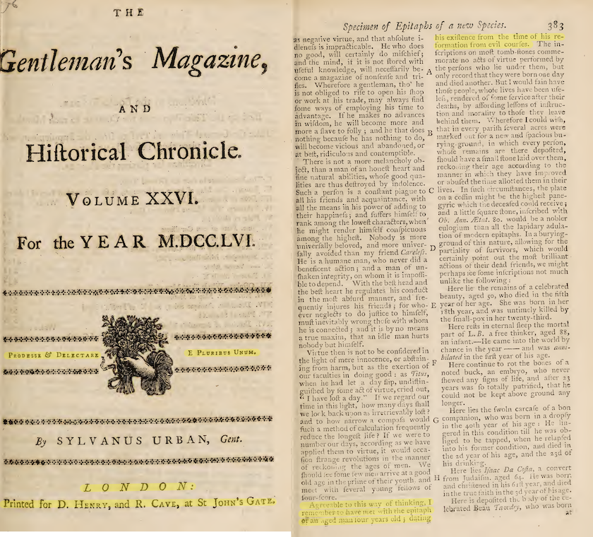
Figure 3: Two pages from The Gentleman’s Magazine - Volume XXVI, with several highlighted sections indicating the text used in the OCR results below.
| Google Vision | Tesseract |
|---|---|
| PRODESSE & DELICTARI E PLURIBUS UNUM. |
Propesse & DErEecTARE E Prvurrsavs UNUM. |
| LONDON: Printed for D. Henry, and R. Cave, at St John’s GATE. |
EON DO #: Printed for D. Hznry, and R. Cave, at St Joun’s GaTE. |
| as negative virtue, and that abſolute in his exiſtence from the time of his re- dleneſs is impracticable. He who does formation froni evil courſes. The in- […]Agreeable to this way of thinking, I Here is depoſited thi body of the ce- remember to have met with the epitaph lebrated Beau Tawdry, who wis born or an aged man four years old; dating |
Acreeable to this way of thinking, I remember to have met with ehe epitaph oF an uged man tour years old 5 Gating his exiſtence from the time of his re- formation from evil courſes. |
| Combined Method I | Combined Method II |
|---|---|
| PRODESSE & DELICTARI E PLURIBUS UNUM. |
PRODESSE & DELICTARI E PLURIBUS UNUM. |
| L O N D ON: Printed for D. Henry, and R. Cave, at St John’s Gate. |
LONDON: Printed for D. Henry, and R. Cave, at St John’s GATE. |
| Agreeable to this way of thinking, I remember to have met with the epitapha or an aged mau four years old; dating his exiſtence from the time of his re- formation from evil courſes. |
Agreeable to this way of thinking, I remember to have met with the epitaph or an aged man four years old; dating his exiſtence from the time of his re- formation froni evil courſes |
Example 3 demonstrates how columns result in a completely erroneous output from Google Vision. The tool rarely takes vertical text separations into account, and reads across columns instead. Both combined methods allow this issue to be resolved.
The difference between the outputs produced by the two combined methods is minimal. However, the line breaks at the end of the left columns are not present in the output of the second combined method. This method uses the original PDF and, since Google Vision reads across columns, these line breaks were simply not recorded.
Preparation
Prerequisites
Although it is suitable for beginners, this lesson supposes some familiarity with the Python programming language. If you are not already familiar with Python 3, you will better understand the code used here if you work through the Python lesson series first. The Python series will teach you how to install Python 3 and download a text editor where you can write your code.
Sample Dataset
You can work through this lesson with any PDF documents you have to hand. I suggest you use at least two documents since the lesson shows how to OCR several files at once. Place them in a directory named docs_to_OCR, for instance.
Alternatively, you can use the same set of three nineteenth century editions of medieval documents that we will be using as examples throughout this lesson. If you opt to do so, begin by downloading the set of files. Unzip it, rename it docs_to_OCR.
These three documents are copyright-free and available on archive.org.
OCR with Tesseract
Tesseract takes image files as input. If you have PDFs, you can transform them into .tiff files using any image editing tool, ImageMagick for instance. The process of converting PDFs to TIFFs using ImageMagick is detailed in the Programming Historian lesson OCR and Machine Translation.
Alternatively, you can use OCRmyPDF. This software is based on Tesseract but works with PDFs. More information can be found in the Programming Historian lesson Working with batches of PDF files.
Both ImageMagick and OCRmyPDF can be operated from the command line.
If you opt for to use OCRmyPDF, run the following commands after navigating to the docs_to_OCR directory.
First command:
ocrmypdf -l eng+lat --redo-ocr --sidecar
JHS_1872_HenryIVandQueenJoanCanterburyCathedral.txt
JHS_1872_HenryIVandQueenJoanCanterburyCathedral.pdf
JHS_1872_HenryIVandQueenJoanCanterburyCathedral_ocr.pdf
Second command:
ocrmypdf -l eng+enm --redo-ocr --sidecar
Skeat_1881_StSwithunExhumation_MiddleEnglish.txt
Skeat_1881_StSwithunExhumation_MiddleEnglish.pdf
Skeat_1881_StSwithunExhumation_MiddleEnglish_ocr.pdf`
Third command:
ocrmypdf -l eng --redo-ocr --sidecar
Anon_1756_Epitaphs.txt
Anon_1756_Epitaphs.pdf
Anon_1756_Epitaphs_ocr.pdf
With Tesseract, it is necessary to specify the language(s) or script(s) of the text using the -l flag. More than one language or script may be specified by using +. You can find the list of language codes and more information about the language models on the Tesseract GitHub page. Depending on your operating system, you might be required to install language packages separately, as described on OCRmyPDF’s documentation page.
OCRmyPDF creates a new PDF file with an OCR overlay. If you are working with PDFs that already have a (presumably unsatisfactory) OCR overlay, the redo-ocr argument allows for a new overlay to be created. The sidecar argument creates a text file that contains the OCR text found by OCRmyPDF. An alternative to the sidecar argument would be to use another program such as pdftotext to extract the embedded texts from the newly created PDF files.
OCR with Google Vision
Google Cloud Platform setup
To be able to use the Google Vision API, the first step is to set up your project on the Google console. The instructions for each step are linked below. Although the Google Cloud documentation can seem daunting if you are not familiar with API services, the process to create a personal project is relatively straightforward and many of Google’s documentation pages include practical, step-by-step instructions. You can either set up your project with the console interface in your browser (recommended for beginners) or with code, if you wish to integrate these steps directly into your script.
1. Create a new Google Cloud project
Before using any of the Google API services, it is necessary to create a project. Each project can have different APIs enabled and be linked to a different billing account.
2. Link your project to a billing account
To use the API, you will need to link the project to a billing account, even if you are only planning to use the free portion of the service or use any free credits you may have received as a new user.
3. Enable the Cloud Vision API
Google APIs have to be enabled before they are used. To enable the Vision API, you will need to look for it in the Google Cloud API Library. There, you can also browse through the other APIs offered by Google, such as the Cloud Natural Language API which provides natural language understanding technologies, and the Cloud Translation API which allows you to integrate translation into a workflow.
4. Create a Google Cloud Service Account
To make requests to a Google API, you need to use a service account, which is different from your Google user account. A service account is associated to a service account key (see next step). In this step, you will create a service account and grant it access to your project. I suggest you pick ‘Owner’ in the role drop-down menu to grant full access.
5. Download and save a service account key
The service account key is a JSON file which can be created and downloaded from the Google Cloud Console. It is used to identify the service account from which the API requests are coming from. To access the Vision API through Python, you will need to include the path to this file in your code.
In Cloud Storage, data are stored in ‘buckets’. Although it is possible to upload folders or files to buckets in your browser, this step is integrated in the code provided below.
Python Setup
It is always best to create a new virtual environment when you start a Python project. This means that each project can have its own dependencies, regardless of what dependencies other projects need. To do so, you could use conda or venv, for instance.
For this project, I would recommend installing all packages and libraries via conda.
Install the Cloud Storage and Cloud Vision libraries:
conda install -c conda-forge google-cloud-vision
conda install -c conda-forge google-cloud-storage
The code below adapts the code provided in the Google Vision documentation to work with batches instead of individual files, and to save the full-text outputs.
Google Vision takes single files stored in Cloud Storage buckets as input. Therefore, the code iterates through a local directory to upload the file in the Cloud Storage, request the full-text annotation of the PDF, then read the JSON output files stored in the Cloud Storage and save the full-text OCR responses locally.
To begin, you will need to import the libraries (google-cloud-storage and google-cloud-vision) that you just installed, as well as the built-in libraries os, json and glob.
import os
import json
import glob
from google.cloud import vision
from google.cloud import storage
Then, you will need to provide the name of your Google Cloud Storage bucket and the path to your JSON service account key.
bucket_name='BUCKET-NAME'
os.environ['GOOGLE_APPLICATION_CREDENTIALS'] = 'PATH/TO/YOUR/ServiceAccountKey.json'
Then, you can create variables for the different processes needed in the code:
# Instantiate a client for the client libraries 'storage' and 'vision', and the services you want to use, i.e. the DOCUMENT_TEXT_DETECTION of the ImageAnnotator service
storage_client = storage.Client()
vision_client = vision.ImageAnnotatorClient()
bucket = storage_client.get_bucket(bucket_name)
feature = vision.Feature(type_=vision.Feature.Type.DOCUMENT_TEXT_DETECTION)

#The file format used (the alternative is 'image/tiff' if you are working with .tiff image files instead of PDFs).
mime_type = 'application/pdf'

#The number of pages that will be grouped in each json response file
batch_size = 2
The larger the batch size, the faster the progress. However, too large a batch size could cause Python to “crash” if your computer’s memory gets overwhelmed.
Running Google Vision
The first step is to create a function that uploads a file to your Google Cloud Storage bucket and requests the OCR annotation according to the information specified above. The request will create JSON files containing all the OCR information, which will also be stored in your bucket.
This function returns the remote path of the folder where the JSON response files are stored so that they can be easily retrieved in the next step.
def JSON_OCR(input_dir, filename):

    #Create a remote path. The combination of os.path.basename and os.path.normath extracts the name of the last directory of the path, i.e. 'docs_to_OCR'. Using the full path would create many useless nested directories inside your bucket.
    remote_subdir= os.path.basename(os.path.normpath(input_dir))
    rel_remote_path = os.path.join(remote_subdir, filename)

    #Upload file to your Google Cloud Bucket as a blob. The term 'blob' stands for 'Binary Large Object' and is used for storing information.
    blob = bucket.blob(rel_remote_path)
    blob.upload_from_filename(os.path.join(input_dir, filename))

    #Remote path to the file.
    gcs_source_uri = os.path.join('gs://', bucket_name, rel_remote_path)

    #Input source and input configuration.
    gcs_source = vision.GcsSource(uri=gcs_source_uri)
    input_config = vision.InputConfig(gcs_source=gcs_source, mime_type=mime_type)

    #Path to the response JSON files in the Google Cloud Storage. In this case, the JSON files will be saved inside a subfolder of the Cloud version of the input_dir called 'json_output'.
    gcs_destination_uri = os.path.join('gs://', bucket_name, remote_subdir, 'json_output', filename[:30]+'_')

    #Output destination and output configuration.
    gcs_destination = vision.GcsDestination(uri=gcs_destination_uri)
    output_config = vision.OutputConfig(gcs_destination=gcs_destination, batch_size=batch_size)

    #Instantiate OCR annotation request.
    async_request = vision.AsyncAnnotateFileRequest(
    features=[feature], input_config=input_config, output_config=output_config)

    #The timeout variable is used to dictate when a process takes too long and should be aborted. If the OCR process fails due to timeout, you can try and increase this threshold.
    operation = vision_client.async_batch_annotate_files(requests=[async_request])
    operation.result(timeout=180)

    return gcs_destination_uri
Now that the OCR process is complete and the response files are stored in the console, you can create an ordered list containing each “blob” ensuring that they will be read in the correct order.
def l_blobs(gcs_destination_uri):

    #Identify the 'prefix' of the response JSON files, i.e. their path and the beginning of their filename.
    prefix='/'.join(gcs_destination_uri.split('//')[1].split('/')[1:])

    #Use this prefix to extract the correct JSON response files from your bucket and store them as 'blobs' in a list.
    blobs_list = list(bucket.list_blobs(prefix=prefix))

    #Order the list by length before sorting it alphabetically so that the text appears in the correct order in the output file (i.e. so that the first two items of the list are 'output-1-to-2.json' and 'output-2-to-3.json' instead 'output-1-to-2.json' and 'output-10-to-11.json', as produced by the default alphabetical order).
    blobs_list = sorted(blobs_list, key=lambda blob: len(blob.name))

    return blobs_list
Next, we can use this list to extract the full-text annotations of each blob, join them to create the full text, and save it to a local file.
def local_file(blobs_list, filename, output_dir):

    #If the output directory does not exist, create it.
    if not os.path.exists(output_dir):
        os.mkdir(output_dir)

    #Create an empty string to store the text.
    output=''

    #Iterate through the list created in the previous function and extract the 'full_text_response' (i.e. the OCRed text) for each page to append it to the output string.
    for blob in blobs_list:
        json_string = blob.download_as_string()
        response=json.loads(json_string)
        full_text_response = response['responses']

        for text in full_text_response:
            try:
                annotation=text['fullTextAnnotation']
                output+=annotation['text']
            except:
                pass

    #Create the path and name of the output file.
    output_file=os.path.join(output_dir, filename.split('.')[0]+'.txt')

    #Create a file and write the output string.
    f=open(output_file, 'x')
    f.write(output)
    f.close()
The following function executes the entire workflow.
def vision_method(input_dir, output_dir, filename):

    #Assign the remote path to the response JSON files to a variable.
    gcs_destination_uri=JSON_OCR(input_dir, filename)

    #Create an ordered list of blobs from these remote JSON files.
    blobs_list = l_blobs(gcs_destination_uri)

    #Read these blobs one by one to create a full-text string and write it to a local file.
    local_file(blobs_list, filename, output_dir)
Finally, the last function executes the workflow for every PDF file within a given directory.
def batch_vision_method(input_dir, output_dir):
    for filename in os.listdir(input_dir):
        if filename.endswith('.pdf'):
            print(filename)
            vision_method(input_dir, output_dir, filename)
Usage example:
#Directory where the files to be OCRed are located.
input_dir='/PATH/TO/LOCAL/DIRECTORY/docs_to_OCR/'

#Directory where the output text files will be stored.
output_dir='/PATH/TO/LOCAL/DIRECTORY/vision_method_txt/'

batch_vision_method(input_dir, output_dir)
Understanding JSON Ouputs
As explained above, the text-detection API creates JSON files which contain full-text annotations of the input PDF file. In the code above, this full-text annotation is queried from the JSON file and saved as a .txt file to your local output folder. These JSON files contain additional information and can be consulted or downloaded from the json_output subfolder in your storage bucket.
For each page, you will find the following information:
- language(s) detected
- width and height
- full text
For each block, paragraph, and word:
- language(s) detected
- coordinates of the bounding box that “frames” the relevant text
For each character:
- language detected
- the “symbol” detected (i.e. the letter or punctuation mark itself)
Most of this information comes with a confidence score between 0 and 1.
The code block below shows the information for the word “HENRY” in the subtitle of Example 1.
{"property":
{"detectedLanguages":
    [{"languageCode": "en"}]},
"boundingBox":
{"normalizedVertices":
    [{"x": 0.435,
      "y": 0.25},
     {"x": 0.5325,
      "y": 0.25},
     {"x": 0.5325,
      "y": 0.2685185},
     {"x": 0.435,
      "y": 0.2685185}]},
"symbols":
[{"property":
     {"detectedLanguages":
            [{"languageCode": "en"}]},
        "text": "H",
        "confidence": 0.99},
    {"property":
        {"detectedLanguages":
            [{"languageCode": "en"}]},
        "text": "E",
        "confidence": 0.99},
    {"property":
        {"detectedLanguages":
            [{"languageCode": "en"}]},
        "text": "N",
        "confidence": 0.99},
    {"property":
        {"detectedLanguages":
            [{"languageCode": "en"}]},
        "text": "R",
        "confidence": 0.99},
    {"property":
        {"detectedLanguages":
            [{"languageCode": "en"}],
            "detectedBreak":
            {"type": "SPACE"}},
        "text": "Y",
        "confidence": 0.99}],
"confidence": 0.99}
To learn more about JSON and how to query JSON data with the command-line utility jq, consult the Programming Historian lesson Reshaping JSON with jq.
You can also query JSON files stored in the json_output subfolder of your bucket with Python. For instance, if you’d like to know which words have a low confidence score, and which language was detected for these words, you can try running the following code:
#This code only looks at the first two pages of 'JHS_1872_HenryIVandQueenJoanCanterburyCathedral.pdf', but you can of course iterate through all the JSON files.
#Get the data from your bucket as a blob.
page_1_2 = bucket.get_blob('docs_to_OCR/json_output/JHS_1872_HenryIVandQueenJoanCa_output-1-to-2.json')
#Read the blob content as byte.
json_string = page_1_2.download_as_string()
#Turn JSON enconded data into a Python object.
response=json.loads(json_string)

#Consecutive for loops to access the deeply-nested elements wanted.
for page in response['responses']:
    for block in page['fullTextAnnotation']['pages'][0]['blocks']:
        for paragraph in block['paragraphs']:
            for word in paragraph['words']:

                #Condition:
                if word['confidence'] < 0.8:
                    #Since the JSON data provides characters one by one, you need to join them to create the word.
                    word_text = ''.join(symbol['text'] for symbol in word['symbols'])
                    #Discard non-alphabetic characters.
                    if word_text.isalpha():
                        #Not all words have a 'detectedLanguages' attribute. The 'try-except' structure allows you to take them into account.
                        try:
                            print(word_text, '\t', word['confidence'], '\tLanguage Code: ', word['property']['detectedLanguages'][0]['languageCode'])
                        except:
                            print(word_text, '\t', word['confidence'])
Result:
full     0.78   Language Code:  en
A    0.11   Language Code:  en
BRIEF    0.72   Language Code:  en
BENRY    0.7    Language Code:  en
IV   0.76   Language Code:  en
a    0.46   Language Code:  en
And      0.77   Language Code:  en
he   0.77   Language Code:  en
sancta   0.79   Language Code:  la
præ      0.71   Language Code:  la
more     0.79   Language Code:  la
This information could help you correct the text. For instance, it would be possible to output all words whose OCR annotation is below a certain confidence threshold in a different colour for manual verification.
Combining Layout and Character Recognition
Combining the two tools is not as straightforward as it should be since Google Vision, unfortunately, does not allow the user to set a detection area using coordinates before the OCR process takes place. However, there are (at least) two ways to go about it.
- The first is to create a new PDF file where text regions are re-arranged vertically so that Google Vision’s inability to detect complex layouts is no longer a problem. With this method, we can still use the “full-text annotation” from the JSON response file.
- The second method is to use the coordinates of the text blocks detected by Tesseract to select the corresponding words detected by Google Vision. In this case, we have to re-create the text, character by character, instead of using the “full-text annotation”.
Tesseract + Google Vision: Method One
The first combined methods converts a document into a list of images (i.e. each page becomes an image). For each new image, the Tesseract API is used to identify text regions. These text regions are then cut, padded and arranged vertically into a new image. For instance, a page featuring two columns will become an image where the two columns are stacked on top of each other. The new image will therefore be roughly half the width and twice the height as the original. The new images are appended and transformed back into one PDF. This PDF is then processed with the vision_method function defined above.
To create these new PDFs sequenced by regions, three new packages are needed. First, pdf2image converts PDFs to PIL (Python Imaging Library) image objects. Second, tesserocr provides the coordinates of the different text regions. Third, pillow helps us rebuild images for each page according to the coordinates provided by tesserocr. Using conda is the simplest way to install the packages.
conda install -c conda-forge pdf2image
conda install -c conda-forge tesserocr
conda install -c anaconda pillow
Before cutting up the text regions to re-arrange them vertically, it is useful to create a function that adds padding to images. The padding adds space between the text region in the new PDF document. Without it, the close proximity between text regions might lead to OCR errors. It is possible to match the padding to the colour of the background, but I have not found that it significantly improves results. The function takes three arguments: the image, the number of pixels added to each side of the image, and the colour of the padding.
from pdf2image import convert_from_path
from tesserocr import PyTessBaseAPI
from PIL import Image

def add_padding(pil_img, n_pixels, colour):
    width, height = pil_img.size
    new_width = width + n_pixels * 2
    new_height = height + n_pixels * 2
    img_pad = Image.new(pil_img.mode, (new_width, new_height), colour)
    img_pad.paste(pil_img, (n_pixels, n_pixels))
    return img_pad
The next step is to create a function that takes an image of a page as input, uses Tesseract’s API to identify the different text regions, and stores them in a list called ‘regions’. Each element of the list will be a tuple containing an image of one of the regions and a dictionary containing the four coordinates of the region (the ‘x’ and ‘y’ coordinates of the top-left corner, as well as the height and the width). For each region, the image is padded using the function defined above and appended to a list initiated at the beginning of the function.
def list_regions(p):
    lim=[]
    with PyTessBaseAPI() as api:
        api.SetImage(p)
        regions = api.GetRegions()
        for (im, box) in regions:
            img_pad = add_padding(im, 5, "white")
            lim.append(img_pad)
    return lim
With this list of images containing the text regions, we can re-create the page by arranging the regions vertically. The function iterates through the images and records their dimension in order to calculate the dimension of the new page to be created. Since the text regions are stacked vertically, the dimension of the new image will be the sum of the heights and the width of the widest text region. Once the empty image is created, each image is pasted onto it, one below the other.
def page(lim):

    total_height = 0
    max_width = 0

    for img_pad in lim:
        w, h = img_pad.size
        total_height += h
        if w > max_width:
            max_width = w

    page_im = Image.new('RGB', (max_width, total_height), color = "white")
    pre_w = 0
    pre_h = 0

    for img_pad in lim:
        page_im.paste(img_pad, (pre_w, pre_h, pre_w+img_pad.size[0], pre_h + img_pad.size[1]))
        pre_h += img_pad.size[1]


    return page_im
We are now ready to apply this method to all pages of a PDF file. The following function converts each page of the input PDF into a new image, stores those images in a list, and saves them locally as a new PDF stored in a new directory.
def new_file_layout(filename, input_dir, store_dir):

    if not os.path.exists(store_dir):
        os.mkdir(store_dir)

    #Create a path where the output file will be stored.
    new_filepath=os.path.join(store_dir, filename)

    #Convert document in list of images.
    pages = convert_from_path(os.path.join(input_dir, filename))

    #Initiate empty list to store the new version of each page.
    lim_p=[]

    for p in pages:
        lim=list_regions(p)
        page_im=page(lim)
        lim_p.append(page_im)

    lim_p[0].save(new_filepath, "PDF" ,resolution=100.0, save_all=True, append_images=lim_p[1:])
The following function executes the above and OCRs the new PDF with the vision_method defined in the previous section.
def combined_method_I(filename, input_dir, store_dir, output_dir):
    if not os.path.exists(output_dir):
        os.mkdir(output_dir)
    new_file_layout(filename, input_dir, store_dir)
    vision_method(store_dir, output_dir, filename)
Finally, we will execute the workflow for every PDF file within a given directory.
def batch_combined_method_I(input_dir, store_dir, output_dir):
    for filename in os.listdir(input_dir):
        if filename.endswith('.pdf'):
            print(filename)

            combined_method_I(filename, input_dir, store_dir, output_dir)
Usage example:
#Directory where the PDF files to be OCRed are located.
input_dir_cm1='PATH/TO/LOCAL/DIRECTORY/docs_to_OCR'

#Directory where the new sequenced PDF files will be stored.
store_dir_cm1= 'PATH/TO/LOCAL/DIRECTORY/combined_I_pdf/'

#Directory where the output text files will be stored.
output_dir_cm1='/PATH/LOCAL/DIRECTORY/TO/combined_I_txt/'

batch_combined_method_I(input_dir_cm1, store_dir_cm1, output_dir_cm1)
Tesseract + Google Vision: Method Two
The second combined method uses the text region coordinates provided by Tesseract to create text output. We will be extracting any words that fall within the defined regions from the JSON response files we generated earlier using the JSON_OCR function as explained in the Google Vision section.
First, we’ll create a function that will output a dictionary which contains the coordinates of each text region, as well as the height and width of each page. The height and width are necessary for converting the pixel coordinates provided by Tesseract to the normalised coordinates provided by Google Vision.
def region_segmentation(input_dir, filename):

    #Initiate empty dictionary.
    dict_pages={}

    #Convert PDF to list of images.
    pages = convert_from_path(os.path.join(input_dir, filename))

    #Initiate page count.
    pn=0
    for p in pages:
        pn+=1
        with PyTessBaseAPI() as api:
            api.SetImage(p)

            #The "regions" variable is a list of tuples. Each tuple contains an image of a text region and a dictionary containing the coordinates of the same text region.
            regions = api.GetRegions()

            #Assign to a variable the list of dictionaries containing the coordinates of each text region of the page.
            r=[region[1] for region in regions]

            #Add to the dictionary initiated above the page number as key and the list of dictionaries as value.
            dict_pages[pn]=r

            #Add keys and values for the width and height of the page.
            dict_pages[str(pn)+'_width'], dict_pages[str(pn)+'_height']=p.size

    return dict_pages
Then, we can create a function that uses the JSON response files produced by Google Vision to extract the words that fall within the defined text regions (whose coordinates are stored in the dictionary created by the function above).
This function iterates through the pages identified in the JSON files (if you set batch_size = 2, then two pages are processed in each JSON file). For each page, we store the list of JSON blocks in a variable. Using a page counter initiated at the beginning of the function, we retrieve the page’s dimensions (width and height) plus text region coordinates from the dictionary created above.
Tesseract gives four region coordinates in pixels: the x and y coordinates for the top-left corner, as well as the height and length of the text region. For each region, the Tesseract coordinates have to be converted to normalised coordinates, since this is what Google Vision is using. Normalised coordinates give the relative position of a point and are therefore numbers between 0 and 1. To be normalised, an absolute coordinate is divided by the width of the page (for x coordinates) or the height (for y coordinates).
The Google Vision JSON file provides the x and y normalised coordinates for all four corners of each word. The order depends of the orientation of the text. Using the minimum and maximum x and y values ensures that we systematically obtain the top-left and bottom-right corner coordinates of the word box. With the normalised coordinates of the top-left (x1, y1) and bottom-right (x2, y2) corner of a Tesseract region, we obtain the box that words from the Google Vision response file need to “fit” into to be added to the text output for that region. Since we are comparing coordinates provided by different tools; and a one-pixel difference might be key, it could be a good idea to slightly reduce the size of the word box which needs to “fit” into the region box for the word to be added to the text output for that region. Note that “words” include the spaces, punctuation, or line breaks that follow them.
Once these normalised region coordinates are established, we can iterate through each word on a page in the Google Vision JSON file and assess whether it is part of a particular text region. This process is repeated for each text region on each page. The text within each region is appended and written to file when the entire document has been processed.
def local_file_region(blobs_list, dict_pages, output_dir, filename):

    if not os.path.exists(output_dir):
        os.mkdir(output_dir)

    text=''

    #Initiate page count.
    n=1

    #For each page of each JSON file, store the list of text blocks (according to Google Vision), the width and height of the page, and the list of text regions coordinates (according to Tesseract).
    for blob in blobs_list:
        json_string = blob.download_as_string()
        response=json.loads(json_string)

        for page in response['responses']:

            blocks=page['fullTextAnnotation']['pages'][0]['blocks']
            p_width = dict_pages[str(n)+'_width']
            p_height = dict_pages[str(n)+'_height']
            r= dict_pages[n]

            #For each text region, we look through each word of the corresponding page in the JSON file to see if it fits within the region coordinates provided by Tesseract.
            for reg in r:

                x1=reg['x']/p_width
                y1=reg['y']/p_height
                x2=(reg['x']+reg['w'])/p_width
                y2=(reg['y']+reg['h'])/p_height

                for block in blocks:

                    for paragraph in block['paragraphs']:
                        for word in paragraph['words']:
                            try:
                                #The "+O.01" and "-0.01" slightly reduce the size of the word box we are comparing to the region box. If a word is one pixel higher in Google Vision than in Tesseract (potentially due to PDF to image conversion), this precaution ensures that the word is still matched to the correct region.
                                min_x=min(word['boundingBox']['normalizedVertices'][0]['x'], word['boundingBox']['normalizedVertices'][1]['x'], word['boundingBox']['normalizedVertices'][2]['x'], word['boundingBox']['normalizedVertices'][3]['x'])+0.01
                                max_x=max(word['boundingBox']['normalizedVertices'][0]['x'], word['boundingBox']['normalizedVertices'][1]['x'], word['boundingBox']['normalizedVertices'][2]['x'], word['boundingBox']['normalizedVertices'][3]['x'])-0.01
                                min_y=min(word['boundingBox']['normalizedVertices'][0]['y'], word['boundingBox']['normalizedVertices'][1]['y'], word['boundingBox']['normalizedVertices'][2]['y'], word['boundingBox']['normalizedVertices'][3]['y'])+0.01
                                max_y=max(word['boundingBox']['normalizedVertices'][0]['y'], word['boundingBox']['normalizedVertices'][1]['y'], word['boundingBox']['normalizedVertices'][2]['y'], word['boundingBox']['normalizedVertices'][3]['y'])-0.01
                                for symbol in word['symbols']:

                                    #If the word fits, we add the corresponding text to the output string.
                                    if(min_x >= x1 and max_x <= x2 and min_y >= y1 and max_y <= y2):
                                        text+=symbol['text']

                                        try:
                                            if(symbol['property']['detectedBreak']['type']=='SPACE'):
                                                text+=' '
                                            if(symbol['property']['detectedBreak']['type']=='HYPHEN'):
                                                text+='-\n'
                                            if(symbol['property']['detectedBreak']['type']=='LINE_BREAK' or symbol['property']['detectedBreak']['type']=='EOL_SURE_SPACE'):
                                                text+='\n'
                                        except:
                                            pass
                            except:
                                pass
            n+=1

    #Write the full text output to a local text file.
    output_file=os.path.join(output_dir, filename.split('.')[0]+'.txt')

    #Create a file and write the output string.
    f=open(output_file, 'x')
    f.write(text)
    f.close()
To clarify this process and the normalisation of coordinates, let’s focus again on the word “HENRY” from the subtitle of the first example document — Miscellania: Tomb of King Henry IV. in Canterbury Cathedral. The dictionary created with the region_segmentation function provides the following information for the first page of this document:
1: [{'x': 294, 'y': 16, 'w': 479, 'h': 33},
  {'x': 293, 'y': 40, 'w': 481, 'h': 12},
  {'x': 545, 'y': 103, 'w': 52, 'h': 26},
  {'x': 442, 'y': 328, 'w': 264, 'h': 27},
  {'x': 503, 'y': 400, 'w': 143, 'h': 14},
  {'x': 216, 'y': 449, 'w': 731, 'h': 67},
  {'x': 170, 'y': 550, 'w': 821, 'h': 371},
  {'x': 794, 'y': 916, 'w': 162, 'h': 40},
  {'x': 180, 'y': 998, 'w': 811, 'h': 24},
  {'x': 210, 'y': 1035, 'w': 781, 'h': 53},
  {'x': 175, 'y': 1107, 'w': 821, 'h': 490}],
 '1_width': 1112,
 '1_height': 1800
As we can see, Tesseract identified 11 text regions and indicated that this first page was 1112 pixels wide and 1800 pixels high.
The coordinates of the top-left and bottom-right corners of the sixth text region of the page (which contains the subtitle of the text and the word “HENRY”) are calculated as follows by the local_file_region function:
x1 = 216/1112 = 0.1942
y1 = 449/1800 = 0.2494

x2 = (216+731)/1112 = 0.8516
y2 = (449+67)/1800 = 0.2867
To process this text region, our function iterates through each word which appears in the JSON block corresponding to this page and checks if it “fits” in this region. When it gets to the word “HENRY”, the function checks the coordinates of the word, which, as we have seen in the JSON section, are:
x: 0.435, y: 0.25
x: 0.5325, y: 0.25
x: 0.5325, y: 0.2685185
x: 0.435, y: 0.2685185
Using the minimum and maximum x and y values, the function calculates that the top-left corner is (0.435, 0.25) and the bottom-right is (0.5325, 0.2685185). With these coordinates, the function assesses if the word “HENRY” fits within the text region. This is done by checking that the x coordinates (0.435 and 0.5325) are both between 0.1942 and 0.8516, and the y coordinates (0.25 and 0.2685185) are both between 0.2494 and 0.2867. Since this is the case, the word “HENRY” is added to the text string for this region.
The following function executes the entire workflow. First, it generates an ordered list of response JSON from Google Vision, just as it would if we were using Google Vision alone. Then, it generates the dictionary containing the Tesseract coordinates of all text regions. Finally, it uses the local_file_region function defined above to create the text output.
def combined_method_II(input_dir, output_dir, filename):
    gcs_destination_uri=JSON_OCR(input_dir, filename)
    blobs_list=l_blobs(gcs_destination_uri)
    dict_pages=region_segmentation(input_dir, filename)
    local_file_region(blobs_list, dict_pages, output_dir, filename)
The following function executes the workflow for every PDF file within a given directory:
def batch_combined_method_II(input_dir, output_dir):
    for filename in os.listdir(input_dir):
        if filename.endswith('.pdf'):
            print(filename)
            combined_method_II(input_dir, output_dir, filename)
Usage example:
#Directory where PDF files to be OCRed are located.
input_dir_cm2='PATH/TO/LOCAL/DIRECTORY/docs_to_OCR'

#Directory where the output text files will be stored.
output_dir_cm2='/PATH/LOCAL/DIRECTORY/TO/combined_II_txt/'

batch_combined_method_II(input_dir_cm2, output_dir_cm2)
Conclusions
When undertaking digital research projects in the humanities, and more so when dealing with historical sources, it is rare to encounter tools that were designed with your material in mind. Therefore, it is often useful to consider whether several different tools are interoperable, and how combining them could offer novel solutions.
This lesson combines Tesseract’s layout recognition tool with Google Vision’s text annotation feature to create an OCR workflow that will produce better results than Tesseract or Google Vision alone. If training your own OCR model or paying for a licensed tool is not an option, this versatile solution might be a cost-efficient answer to your OCR problems.