Contents
- Lesson Goals
Lesson Goals
In this lesson, you will learn how to create a web map based on that data. By the end of this lesson, you will be able to:
- Manipulate tabular data programmatically to extract geonames and create location-based data
- Convert tabular data into a meaningful geographic data structure
- Understand and apply the basic concepts of web mapping to design your own web map
Getting Started
Initial Setup
This lesson uses:
Optional: If you wish to follow along with pre-made scripts you can find them in this directory.
To set up your working environment:
- Create a directory for this project where you will keep all of your scripts and files that you will work from
- If you have a text editor where you can work from the directory of your project, import that directory. You can use editors such as TextWrangler for OS X, Notepad++ for Windows, or Sublime Text. If you are using a code editor such as Sublime Text, to import the folder you could drag and drop the folder that you want to work from into your editor window. Once you’ve done that, the directory will appear on the left hand sidebar as you root folder. If you click on your folder, you’ll be able to see the contents of your folder. Importing a folder allows you to easily work with the files in your project. If you need to work with multiple files and directories in directories, this will make it easier to search through these files, switch between them while you’re working and keep you organized.
- (Optional) It is recommended to use a Python virtual environment to store the dependencies and versions required for your specific project.
Getting Data: Download the CSV
We’re going to start with a plain comma-separated values (CSV) data file and create a web map from it.
The data file can be downloaded here. You can grab this by either opening the link in your browser and saving the page, or you can use the curl command from your command line:
curl -O https://programminghistorian.org/assets/mapping-with-python-leaflet/census.csv
The original source of this data is from the Greater London Authority London Datastore.
Geocoding with Python
Geocode the placenames in the CSV using Geopy, Pandas
Now that we have data, we will use this as our source to make a web map. Web maps typically represent locations and features from geographic data formats such as geoJSON and KML. Every location in a geographic data file can be considered to have geometry (such as points, lines, polygons) as well as additional properties. Web maps typically understand locations as a series of coordinates. For example, 43.6426,-79.3871 would represent the exact coordinates of the CN Tower in Toronto.
In our data file, we have a list of placenames in our CSV data (the Area Name column), but no coordinates. What we want to do then is to somehow generate coordinates from these locations. This process is called geocoding.
So here is our first problem to solve: how can we geocode placenames? How could we take an entry such as “CN Tower” and add the coordinates 43.6426,-79.3871 to it automatically?
To clarify, we need to figure out how to gather coordinates for a location for each row of a CSV file in order to display these locations on a web map.
There’s a simple way to do this: you can look up a coordinate online in Google Maps and put each coordinate in your spreadsheet manually. But, if you had 5,000 points the task becomes a little bit more daunting. If you’re faced with a repetitive task, it might be worthwhile to approach it programmatically.
If you’re familiar with Programming Historian, you might have already noticed that there are many lessons available on how to use Python. Python is a great beginner programming language because it is easy to read and happens to be used a lot in GIS applications to optimize workflows. One of the biggest advantages to Python is the impressive amount of libraries which act like pluggable tools to use for many different tasks. Knowing that this is a good programmatic approach, we’re now going to build a Python script that will automate geocode every address for us.
Geopy is a Python library that gives you access to the various geocoding APIs. Geopy makes it easy for Python developers to locate the coordinates of addresses, cities, countries, and landmarks across the globe using third-party geocoders and other data sources. Geopy includes geocoders built by OpenStreetMap Nominatim, ESRI ArcGIS, Google Geocoding API (V3), Baidu Maps, Bing Maps API, Yahoo! PlaceFinder, Yandex, IGN France, GeoNames, NaviData, OpenMapQuest, What3Words, OpenCage, SmartyStreets, geocoder.us, and GeocodeFarm geocoder services.
Pandas is another python library that we will use. It’s very popular library amongst scientists and mathematicians to manipulate and analyse data.
Finally, Pip is a very useful package manager to help you install things like Geopy and Pandas! If you’ve already installed Python and installed pip, type pip list to see if you already have the geopy and pandas packages installed. If you do not have pip installed, you can download get-pip.py, then from your command line go to the directory where get-pip.py is located and run
python get-pip.py
For the most up to date instructions, you can visit pip’s installation manual.
To install Geopy and Pandas, open your command line (using this lesson as a guideline if necessary) and install the Geopy and Pandas libraries:
On OS X or Linux, the following commands will install the necessary packages:
pip install numpy
pip install python-dateutil
pip install pytz
pip install geopy
pip install pandas
Note: We are installing numpy, python-dateutil, and pytz because pandas requires them.
For Windows, you may need to install Microsoft Visual C++ Compiler for Python. Set the environmental variables to recognize python and pip from the command line:
setx  PATH "%PATH%;C:\Python27"
setx  PATH "%PATH%;C:\Python27\Scripts"
If you keep getting an error when you’re trying to install these libraries, you may need to use sudo pip install instead of just pip install. You may also need to upgrade your libraries if you’ve installed them earlier and you find that you’re encountering an error when using Python (i.e. an ImportError). In order to do so, the following command works:
pip install python --upgrade
Repeat for the other dependencies listed above.
Now we’re going to start building our script. We’re going to go through the script, line by line, and then run it through the command line at the end. To get started, open your text editor and save your blank document as a python script (name it geocoder.py). For the first part of your Python script, you will want to import your libraries and your data:
import geopy
import pandas
from geopy.geocoders import Nominatim
# versions used: geopy 2.2.0, pandas 1.3.3, python 3.7.5
In the code above, we are importing the different Python libraries that we will need to use later on in our script. We import geopy, specifically the geopy.geocoders that we will call on later which is Nominatim and Google Maps V3 API, and we import pandas.
Then you want to create a function main() that reads your input CSV.
import geopy
import pandas
from geopy.geocoders import Nominatim
# versions used: geopy 2.2.0, pandas 1.3.3, python 3.7.5

def main():
	io = pandas.read_csv('census-historic-population-borough.csv', index_col=None, header=0, sep=",")
We are first using pandas’ pre-existing read_csv() function to open the CSV file. We pass the filepath to our data file in the first parameter, ‘census-historic-population-borough.csv’. If it was in a folder called ‘data’, you would put ‘data/census-historic-population-borough.csv’. The second parameter, index_col=None, will number the rows to generate the index without using any column. If we use index_col=0, it indexes the first column in your data as the row name. The third parameter, header=0, indicates that there is a header row, which is the first line of the spreadsheet (Note: Python uses “0” instead of “1” to indicate the first value in an index). The fourth parameter sep="," is where you indicate delimiter symbol that is used to split data into fields. Since are using a comma separated values data format, we need to indicate that we are using a comma to split our data.
There are many other parameters you can use. A full list is available in the pandas documentation on the read_csv() function.
Next, we anticipate that when we geocode the csv we will get points in the format of (latitude, longitude). If we only want the latitude value of the point in a csv column, we will define a function to isolate that value. The same can be done for our longitude value.
import geopy
import pandas
# versions used: geopy 2.2.0, pandas 1.3.3, python 3.7.5

def main():
  io = pandas.read_csv('census-historic-population-borough.csv', index_col=None, header=0, sep=",")

def get_latitude(x):
  return x.latitude

def get_longitude(x):
  return x.longitude
Next, select the geolocator you want to use. Here we’re creating two geolocators: Open Street Map’s Nominatim and Google’s Geocoding API. Here’s a quick comparison:
| Geolocator | Nominatim() |
|---|---|
| affiliation | OpenStreetMap |
| application use | single-threaded applications, can only run geolocator one process at a time |
| capabilities for app development | can geocode based on user-input |
| request limit | 1 request/s or timeout |
| performance test on census data | 33.5s |
You can also choose a different geolocator from the list found in the geopy documentation. GoogleV3 is a geocoder compatible with geopy, it is a reliable geolocator choice because of their large geographic data coverage. However, since July 2018 an API key is required, and you need to enable billing in Google Cloud to use it. For more information about choosing geolocators, you can follow the discussion in the geopy repository on Github.
To use a geolocator, import them and assign a variable name (in this case we use the name geolocator):
import geopy
import pandas
from geopy.geocoders import Nominatim
# versions used: geopy 2.2.0, pandas 1.3.3, python 3.7.5

def main():
  io = pandas.read_csv('census-historic-population-borough.csv', index_col=None, header=0, sep=",")

  def get_latitude(x):
    return x.latitude

  def get_longitude(x):
    return x.longitude

geolocator = Nominatim()
Finally, using pandas you want to create a column in your spreadsheet called ‘latitude’. The script will read the existing ‘Area_Name’ data column, run the geopy geolocator on the column using pandas’ apply function, and generate a latitude coordinate in that column. The same transformation will occur in the ‘longitude’ column. Once this is finished it will output a new CSV file with those two columns:
import geopy
import pandas
from geopy.geocoders import Nominatim
# versions used: geopy 2.2.0, pandas 1.3.3, python 3.7.5

def main():
  io = pandas.read_csv('census-historic-population-borough.csv', index_col=None, header=0, sep=",")

  def get_latitude(x):
    return x.latitude

  def get_longitude(x):
    return x.longitude

  geolocator = Nominatim()

  geolocate_column = io['Area_Name'].apply(geolocator.geocode)
  io['latitude'] = geolocate_column.apply(get_latitude)
  io['longitude'] = geolocate_column.apply(get_longitude)
  io.to_csv('geocoding-output.csv')
If we didn’t have the .apply(get_latitude) part of the code, we’d get the full point data. For instance, if we were again geocoding the CN Tower and used just .apply(geolocator.geocode), we would get 43.6426,-79.3871 in our column. Adding the additional .apply(get_latitude) would mean that we’d only get 43.6426 in our column.
To finish off your code, it’s good practice to make your python modular, that way you can plug it in and out of other applications (should you want to use this script as part of another program). This is what your final python script should look like:
import geopy
import pandas
from geopy.geocoders import Nominatim
# versions used: geopy 2.2.0, pandas 1.3.3, python 3.7.5

def main():
  io = pandas.read_csv('census-historic-population-borough.csv', index_col=None, header=0, sep=",")

  def get_latitude(x):
    return x.latitude

  def get_longitude(x):
    return x.longitude

  geolocator = Nominatim(user_agent="email@email.com")

  geolocate_column = io['Area_Name'].apply(geolocator.geocode)
  io['latitude'] = geolocate_column.apply(get_latitude)
  io['longitude'] = geolocate_column.apply(get_longitude)
  io.to_csv('geocoding-output.csv')

if __name__ == '__main__':
  main()
Do you have the script saved and ready to go? Good. Run the script from your command line by typing:
python geocoder.py
It takes a few seconds and may take longer depending on the geolocator you use. Once the script finishes running, you should have coordinates for every Area_Name.
Tip 1: If you want to pass the filenames from the command line rather than changing the input file name in the python script everytime, you can import the python ‘sys’ library to pass through arguments. Your code might look like this:
import geopy, sys
import pandas
from geopy.geocoders import Nominatim
# versions used: geopy 2.2.0, pandas 1.3.3, python 3.7.5

inputfile=str(sys.argv[1])
namecolumn=str(sys.argv[2])

def main():
  io = pandas.read_csv(inputfile, index_col=None, header=0, sep=",")

def get_latitude(x):
  return x.latitude

  def get_longitude(x):
    return x.longitude

  geolocator = Nominatim()

  geolocate_column = io[namecolumn].apply(geolocator.geocode)
  io['latitude'] = geolocate_column.apply(get_latitude)
  io['longitude'] = geolocate_column.apply(get_longitude)
  io.to_csv('geocoding-output.csv')

if __name__ == '__main__':
  main()
To run your python script your command would look like this:
python geocoder.py census-historic-population-borough.csv Area_Name
Tip 2: If you run geocoder.py too many times you might get a timeout error.
The error will look like this if you use the Nominatim geocoder:
geopy.exc.GeocoderTimedOut: Service timed out
To address the timeout error, you could add the parameter timeout, which specifies the time, in seconds, to wait for the geocoding service to respond before raising a geopy.exc.GeocoderTimedOut exception. So your geolocator declaration will look like this:
geolocator = Nominatim(user_agent="email@email.com", timeout=5)
Transforming Data with Python
Making GeoJSON
Now that you have a spreadsheet full of coordinate data, we can convert the CSV spreadsheet into a format that web maps like, like GeoJSON. GeoJSON is a web mapping standard of JSON data. There are a couple of ways to make GeoJSON:
The easiest, recommended way is to use a UI tool developed by Mapbox called geojson.io. All you have to do is click and drag your csv file into the data window (the right side of the screen, next to the map), and it will automatically format your data into GeoJSON for you. You can select the ‘GeoJSON’ option under ‘Save.’ Save your GeoJSON file as census.geojson.
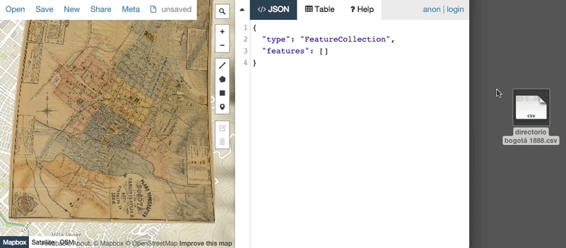
Drag and Drop GeoJSON creation!
Image Credit: with permission from Mauricio Giraldo Arteaga, NYPL Labs
You can also do it from the command line, using the csv2geojson library that powers geojson.io.
Test this data out by importing it again into geojson.io. You should see points generated in the preview window. That’s your data!
You finally have GeoJSON… but you need to do some cleaning!
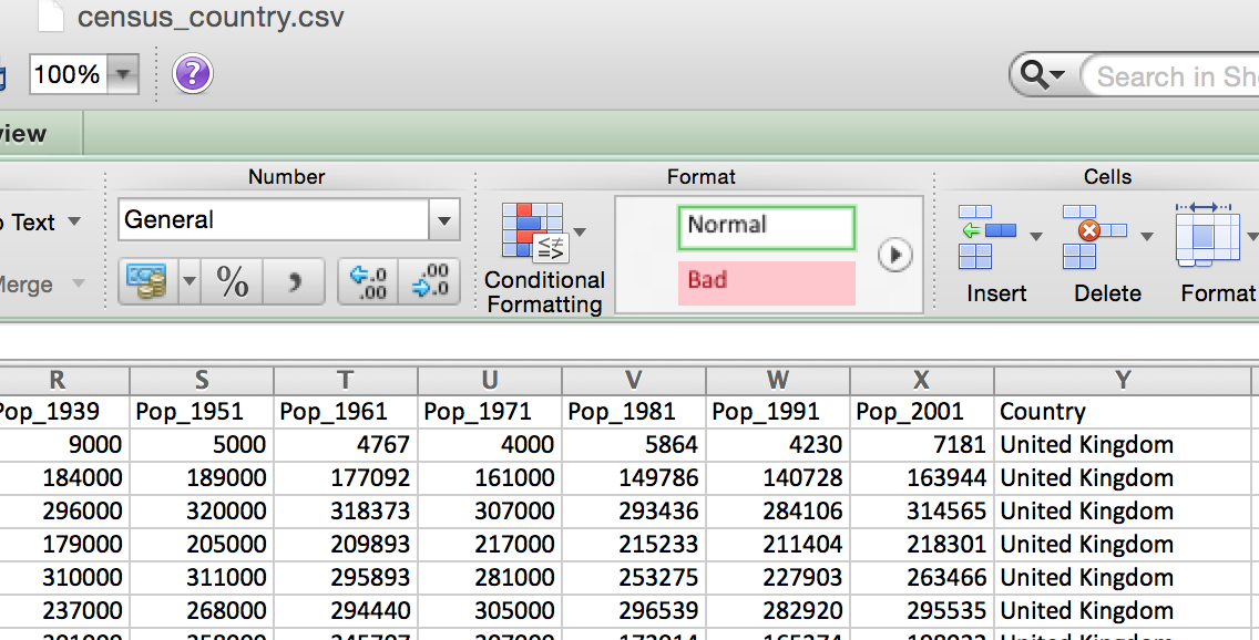
If you’ve tested your GeoJSON data, you might notice that not every point is geolocated correctly. We know that every Area_Name is a borough of London, but points appear all over United Kingdom, and some aren’t located even in the country.
To make the results more accurate, save another copy of the census-historic-population-borough.csv file, calling it census_country.csv and include an additional column called ‘Country’ and put ‘United Kingdom’ in every row of your data. For even greater accuracy add ‘City’ and put ‘London’ in every row of your data to provide additional context for your data.
A new Country column
Make a copy of your geocoder.py python script, calling it geocoder-helpercolumn.py. Remove the following lines:
  geolocate_column = io[namecolumn].apply(geolocator.geocode)
  io['latitude'] = geolocate_column.apply(get_latitude)
  io['longitude'] = geolocate_column.apply(get_longitude)
and replacing it with the following that combines the Area_Name and Country or City column to geocode your data:
  io['helper'] = io['Area_Name'].map(str) + " " + io['Country'].map(str)
  geolocate_column = io['helper'].apply(geolocator.geocode)
  io['latitude'] = geolocate_column.apply(get_latitude)
  io['longitude'] = geolocate_column.apply(get_longitude)
Note that we added the .map(str) function. This is a pandas function that is allowing you to concatenate two DataFrame columns into a new, single column (helper) using the syntax format:
df['newcol'] = df['col1'].map(str) + df['col2'].map(str)
You will also want to comment out and commenting out namecolumn=str(sys.argv[2]) since we are now directly specifying the column that we are using in the script.
Your final script should look like this:
import geopy, sys
import pandas
from geopy.geocoders import Nominatim

inputfile=str(sys.argv[1])
# namecolumn=str(sys.argv[2])

def main():
  io = pandas.read_csv(inputfile, index_col=None, header=0, sep=",")

  def get_latitude(x):
    return x.latitude

  def get_longitude(x):
    return x.longitude

  # geolocator = Nominatim(timeout=5)
  # uncomment the geolocator you want to use
  # change the timeout value if you get a timeout error, for instance, geolocator = Nominatim(timeout=60)
  io['helper'] = io['Area_Name'].map(str) + " " + io['Country'].map(str)
  geolocate_column = io['helper'].apply(geolocator.geocode)
  io['latitude'] = geolocate_column.apply(get_latitude)
  io['longitude'] = geolocate_column.apply(get_longitude)
  io.to_csv('geocoding-output-helper.csv')

if __name__ == '__main__':
  main()
Which you can now run by using the command:
python geocoder-helpercolumn.py census_country.csv
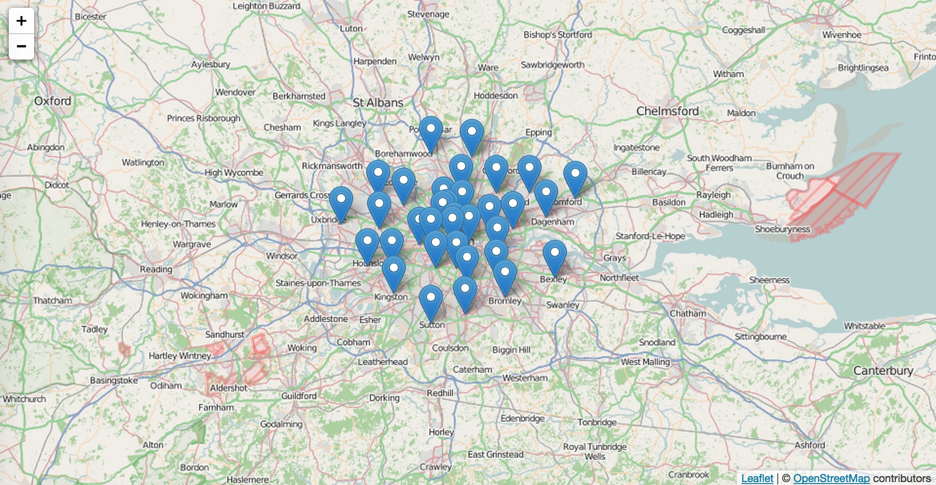
Turn your clean data into GeoJSON by saving it as census.geojson and test it out at geojson.io. Remember, drag the new CSV you created (census_country.csv into the window to create that beautiful JSON). Do the results look better now? Good!
Using Leaflet to Create a Web Map
I now have clean GeoJSON data. Lets make a map!
Setup a test web server to test out our maps. A web server is used to serve content from your directory to your browser.
If you’re in your working directory, from the command line, run:
python -m SimpleHTTPServer or python3 -m http.server (for Python3)
SimpleHTTPServer is a Python module. If you want to change the server to port 8080 (or any other port), use
python -m SimpleHTTPServer 8080 or python3 -m http.server 8080 (for Python3)
In your browser go to http://localhost:8080 and you should see the files you’ve been working with so far.
Now in your text editor open a new document and save it as an html file (mymap.html). If you want to do a quick test, copy and paste the text below, refresh your http://localhost:8080 and open the html file in your browser.
<!DOCTYPE html>
<head>
<link rel="stylesheet" href="http://cdn.leafletjs.com/leaflet-0.6.4/leaflet.css" />
<script src="http://cdn.leafletjs.com/leaflet-0.6.4/leaflet.js"></script>
<script src="https://code.jquery.com/jquery-2.1.4.min.js"></script>
<style>
#my-map {
width:960px;
height:500px;
}
</style>
</head>
<body>
<div id="my-map"></div>
<script>
window.onload = function () {
var basemap = L.tileLayer('http://{s}.tile.osm.org/{z}/{x}/{y}.png', {
attribution: '© <a href="http://osm.org/copyright">OpenStreetMap</a> contributors'
});
$.getJSON("census.geojson", function(data) {
var geojson = L.geoJson(data, {
onEachFeature: function (feature, layer) {
layer.bindPopup(feature.properties.Area_Name);
}
});
var map = L.map('my-map')
.fitBounds(geojson.getBounds());
// .setView([0.0,-10.0], 2);
basemap.addTo(map);
geojson.addTo(map);
});
};
</script>
</body>
</html>
Do you see a map now? Good! If not, you can troubleshoot by inspecting the browser, or by going back and retracing your steps.
What did I just make?
You made a web map! Web maps use map tiles, which are pixel based images (rasters) of maps that contain geographical data. This means that each pixel of a map tile has been georeferenced, or assigned a coordinate based on the location that they represent. When you zoom in and out of a web map, you are getting a whole new set of tiles to display at each zoom level. GeoJSON (which you are now familiar with) is a widely used data standard for web mapping. In our example, we are using an open-source Javascript library called Leaflet to help us build our web map. The benefits of using an open-source library such as Leaflet is the flexibility you get and with developing and customizing your map, without worry of the technology being deprecated or no longer supported that is beyond your control. With frameworks like Leaflet or Google Maps Javascript API, you’re not building a map completely from scratch, rather, you’re using pre-written functions and controls that helps you customize your own map in code.
Lets go through what each part of the code is doing. But first, it’s best practice to maintain your html, css, js in different files so that the web map’s content, presentation and behaviour layers are kept separate (though it’s not always possible). This adds a bit more structure to your code, making it easier for you and others to understand. It will be easier to focus on certain parts of the code when you’re going back and making changes. So here is our code split into three files:
mymap.html
<!DOCTYPE html>
<head>
<link rel="stylesheet" href="http://cdn.leafletjs.com/leaflet-0.6.4/leaflet.css" />
<script src="http://cdn.leafletjs.com/leaflet-0.6.4/leaflet.js"></script>
<script src="https://code.jquery.com/jquery-2.1.4.min.js"></script>
<link rel="stylesheet" href="style.css" />
</head>

<body>
	<div id="my-map"></div>
</body>
<script src='leafletmap.js'></script>

</html>
style.css
#my-map {
	width:960px;
	height:500px;
}
leafletmap.js
window.onload = function () {
var basemap = L.tileLayer('http://{s}.tile.osm.org/{z}/{x}/{y}.png', {
attribution: '© <a href="http://osm.org/copyright">OpenStreetMap</a> contributors'
});
$.getJSON("census.geojson", function(data) {
var geojson = L.geoJson(data, {
onEachFeature: function (feature, layer) {
layer.bindPopup(feature.properties.Area_Name);
}
});
var map = L.map('my-map')
.fitBounds(geojson.getBounds());
basemap.addTo(map);
geojson.addTo(map);
});
};
Seems a bit easier to undestand now, doesn’t it? Now lets look at what the html file is doing.
mymap.html walkthrough
mymap.html
<!DOCTYPE html>
<head>
<link rel="stylesheet" href="http://cdn.leafletjs.com/leaflet-0.6.4/leaflet.css" />
<script src="http://cdn.leafletjs.com/leaflet-0.6.4/leaflet.js"></script>
<script src="https://code.jquery.com/jquery-2.1.4.min.js"></script>
<link rel="stylesheet" href="style.css" />
</head>
The above code is the first section, or header of your html document. We are linking to the external javascript library and css stylesheets provided by leaflet. We’re also linking to our own stylesheet, style.css.
<body>
	<div id="my-map"></div>
</body>
<script src='leafletmap.js'></script>

</html>
Next, we’re declaring the body and where you want the map to go on your page. We’re also linking to our own javascript file, leafletmap.js.
style.css walkthrough
style.css
#my-map {
	width:960px;
	height:500px;
}
There’s a bit of CSS styling here to specify the size of your map. Some optional styling will happen in your javascript file if you’re using the Leaflet library.
leafletmap.js walkthrough
leafletmap.js
window.onload = function () {
var basemap = L.tileLayer('http://{s}.tile.osm.org/{z}/{x}/{y}.png', {
attribution: '© <a href="http://osm.org/copyright">OpenStreetMap</a> contributors'
});
The javascript file is what provides the behaviour, or functionality of our web map. It’s what makes our web map come alive! In the code above, we’re telling the javascript to load when the browser loads. We’re creating our first map layer, which is your basemap. The basemap is the tiles provided by OpenStreetMap that provides places and streetnames found on maps.
	$.getJSON("census.geojson", function(data) {

    var geojson = L.geoJson(data, {
      onEachFeature: function (feature, layer) {
        layer.bindPopup(feature.properties.Area_Name);
      }
    });
Next, we’re loading our data as another map layer, census.geojson. This data will have additional properties: each point of data is represented by an icon. It will look and behave like a popup so that when you click on the icon it will load information from your data file (in this case, the Area_Name).
   var map = L.map('my-map')
    .fitBounds(geojson.getBounds());

    basemap.addTo(map);
    geojson.addTo(map);
  });

};
Now we’re creating the view for our map. The boundary for our map will be based on the range of our data points in census.geojson. You can also manually set your your viewport by using the setView property. For example, if you’re using .setView([0.0,-10.0], 2) , the viewport coordinates ‘[0.0,-10.0], 2’ means that you’re setting the centre of the map to be 0.0, -10.0 and at a zoom level of 2.
My Web Map
Finally, the map layers you created will be added to your map. Put it all together and hurrah, you’ve got your web map! Now lets play around with it. The following five exercises give you tasks to do to learn some of the other elements, with answers provided.
Exercise 1: Default Viewports
Let’s change the map to use a viewport to 51.505 latitude, -0.09 longitude with a zoom level 9. To do this, we just need to edit one file: leafletmap.js.
window.onload = function () {
var basemap = L.tileLayer('http://{s}.tile.osm.org/{z}/{x}/{y}.png', {
attribution: '© <a href="http://osm.org/copyright">OpenStreetMap</a> contributors'
});
$.getJSON("census.geojson", function(data) {
var geojson = L.geoJson(data, {
onEachFeature: function (feature, layer) {
layer.bindPopup(feature.properties.Area_Name);
}
});
var map = L.map('my-map')
//.fitBounds(geojson.getBounds());
.setView([51.505,-0.09], 9);
//EDIT HERE
basemap.addTo(map);
geojson.addTo(map);
});
};
What we’ve done there is changed the .fitBounds to .setView, with the various options mentioned above. Try reloading the file, and you’ll see it loads to the correct place.
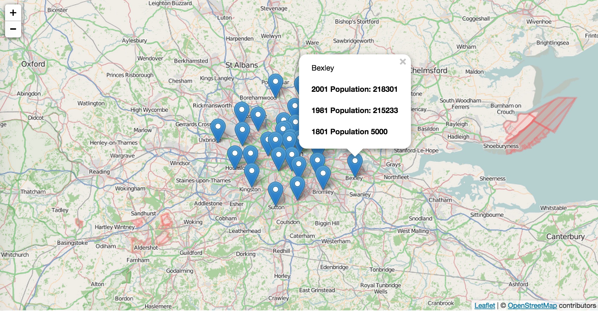
Exercise 01
Exercise 2: Marker Properties
Now let’s add the 2001, 1981 and 1991 population property to each marker popup. You can use HTML to style your popup window. To do so, we again need to edit the javascript.
window.onload = function () {
var basemap = L.tileLayer('http://{s}.tile.osm.org/{z}/{x}/{y}.png', {
attribution: '© <a href="http://osm.org/copyright">OpenStreetMap</a> contributors'
});
$.getJSON("census.geojson", function(data) {
var geojson = L.geoJson(data, {
onEachFeature: function (feature, layer) {
layer.bindPopup(feature.properties.Area_Name + '<p><b> 2001 Population: ' + feature.properties.Pop_2001 + '</b></p>' + '<p><b> 1981 Population: ' + feature.properties.Pop_1981 + '</b></p>' + '<p><b> 1801 Population ' + feature.properties.Pop_1801 + '</b></p>');
//EDIT HERE
}
});
var map = L.map('my-map')
//.fitBounds(geojson.getBounds());
.setView([51.505,-0.09], 9);
basemap.addTo(map);
geojson.addTo(map);
});
};
What we’ve done here is edit the onEachFeature function, which gets called for each feature (in this case, each marker popup) to add additional information about each marker contained in our census.geojson data. To add attribute information from our census.geojson file, we use the convention feature.properties.ATTRIBUTE_NAME to access the population data. In this case, we are adding feature.properties.Pop_2001, feature.properties.Pop_1981, and feature.properties.Pop_1801, and adding a bit of styling with html for readability.
Exercise 02
Exercise 3: Change Data Source
Change the data source to a different dataset, as an example you can use the stations.geojson file.
To do this, we need to edit the javascript file.
window.onload = function () {
var basemap = L.tileLayer('http://{s}.tile.osm.org/{z}/{x}/{y}.png', {
attribution: '© <a href="http://osm.org/copyright">OpenStreetMap</a> contributors'
});
$.getJSON("stations.geojson", function(data) {
var geojson = L.geoJson(data, {
onEachFeature: function (feature, layer) {
layer.bindPopup(feature.properties.name + '<p><b> Line: ' + feature.properties.line + '</b></p>');
//EDIT HERE
}
});
var map = L.map('my-map')
.fitBounds(geojson.getBounds());
// .setView([51.505,-0.09], 9);
// EDIT HERE
basemap.addTo(map);
geojson.addTo(map);
});
};
Since we’re loading a new dataset, we need a new view for our map. First, we’ve replaced census.geojson with stations.geojson to our $getJSON request. Next, we add the attribute information found in our stations.geojson file, including the name (feature.properties.name) and line (features.properties.line). Finally, we are using the .fitBounds function so that the viewport automatically centers on our new set of data points.
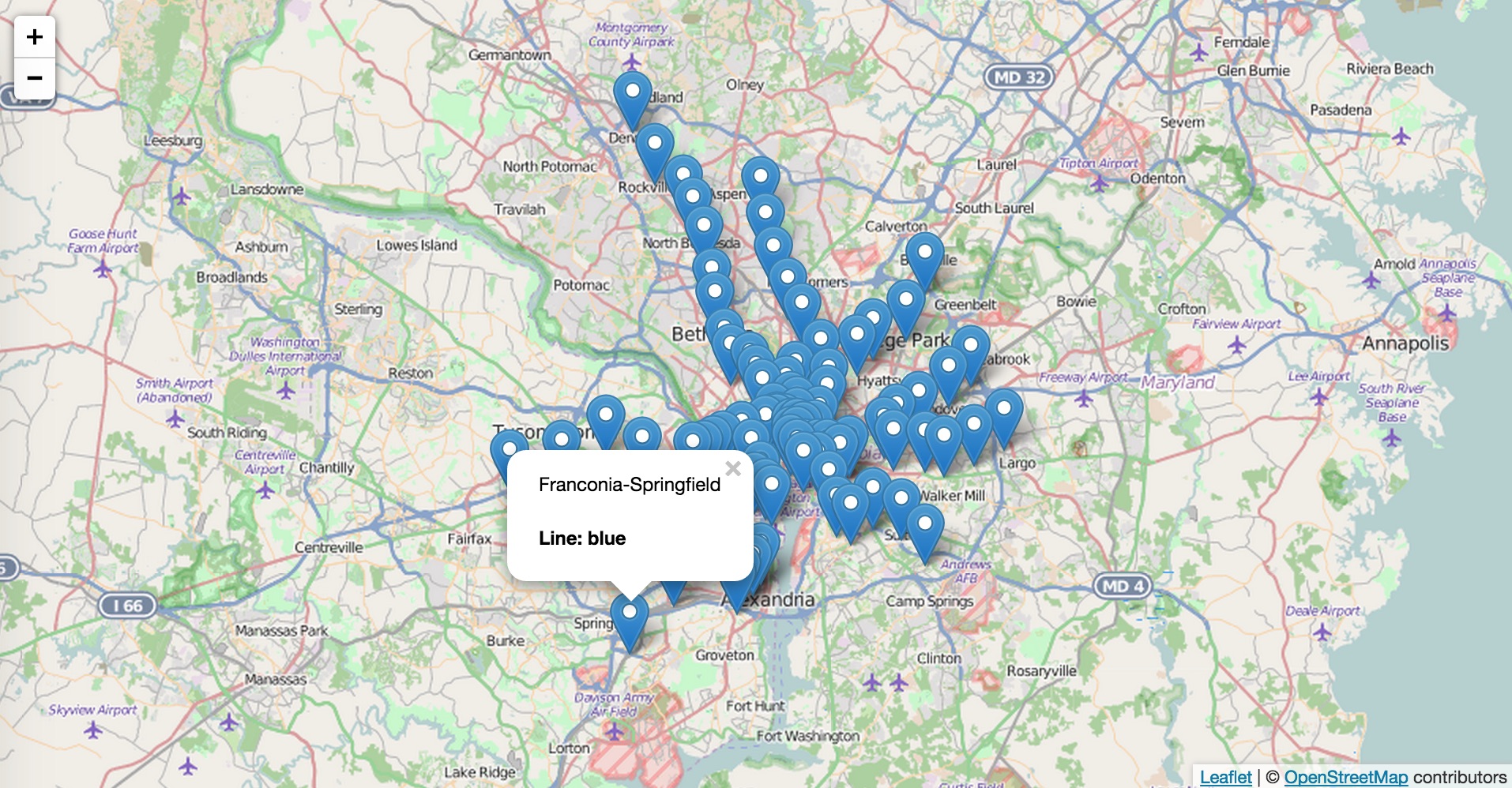
Exercise 03
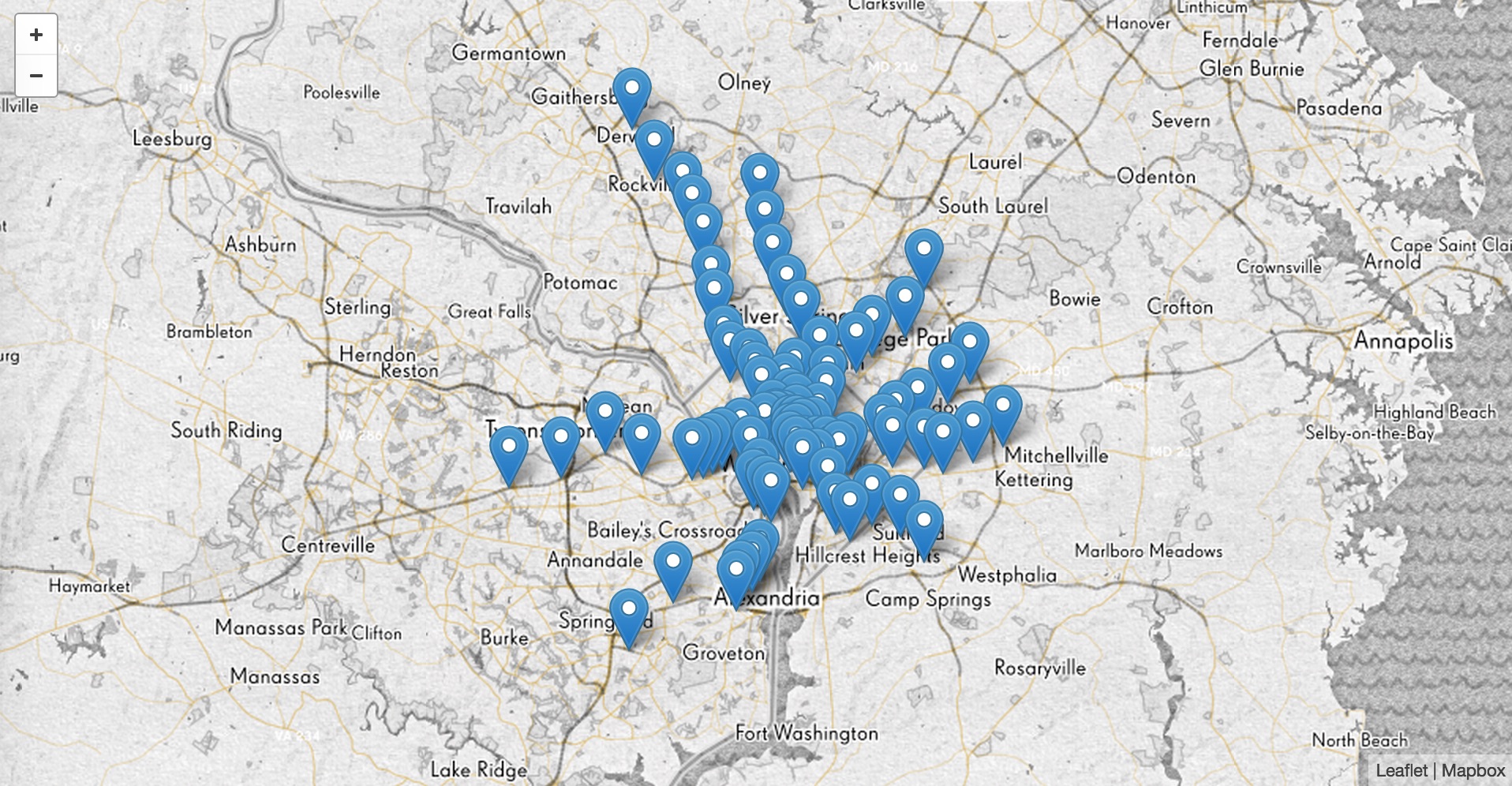
Exercise 4: Custom Basemap
Change your data source back to census.geojson. Change your basemap layer to a mapbox tileset. You need to get a Mapbox account, create a map or style and get your Mapbox API access token.
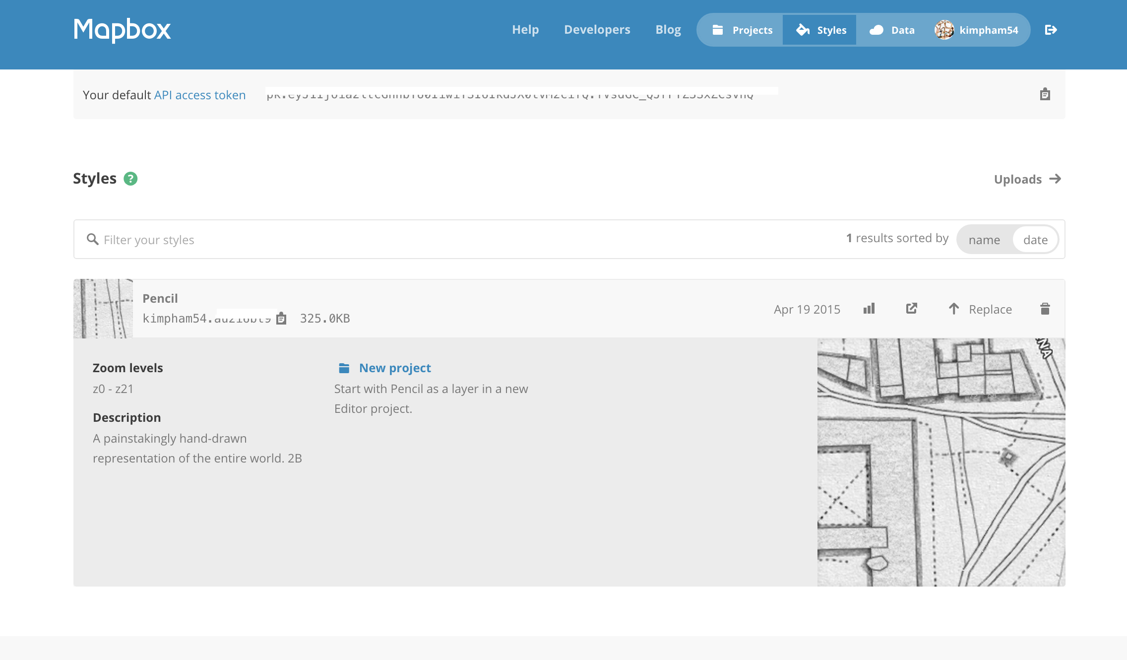
Mapbox API
First, you will need to add a reference to the mapbox javascript and css libraries:
<!DOCTYPE html>
<head>
<link rel="stylesheet" href="http://cdn.leafletjs.com/leaflet-0.6.4/leaflet.css" />
<script src="http://cdn.leafletjs.com/leaflet-0.6.4/leaflet.js"></script>
<script src="https://code.jquery.com/jquery-2.1.4.min.js"></script>
<!-- EDIT HERE -->
<script src='https://api.mapbox.com/mapbox.js/v2.2.1/mapbox.js'></script>
<link href='https://api.mapbox.com/mapbox.js/v2.2.1/mapbox.css' rel='stylesheet' />
<link rel="stylesheet" href="style.css" />
</head>

<body>
  <div id="my-map"></div>
</body>
<script src='leafletmap.js'></script>

</html>
Then we edit the javascript file:
window.onload = function () {
var basemap = L.tileLayer('http://{s}.tile.osm.org/{z}/{x}/{y}.png', {
attribution: '© <a href="http://osm.org/copyright">OpenStreetMap</a> contributors'
});
// EDIT HERE: get an access token, replace 'YOURTOKENHERE' with something like "pk.eyJ1Ijoia2ltcGhhbTU0IiwiYSI6IkdJX0tvM2cifQ.fVsdGC_QJrFYZ3SxZCsvhQ"
L.mapbox.accessToken = 'YOURTOKENHERE';
// EDIT HERE: add the new baselayer style, replace 'YOURLINKHERE' with something like "kimpham54.au2i6bt9"
var basemap = L.tileLayer('https://api.mapbox.com/v4/kimpham54.au2i6bt9/{z}/{x}/{y}.png?access_token=' + L.mapbox.accessToken, {
attribution: '<a href="https://www.mapbox.com/tos/">Mapbox</a>'
});
$.getJSON("stations.geojson", function(data) {
var geojson = L.geoJson(data, {
onEachFeature: function (feature, layer) {
layer.bindPopup(feature.properties.name + '<p><b> Line: ' + feature.properties.line + '</b></p>');
// EDIT HERE
}
});
var map = L.map('my-map')
.fitBounds(geojson.getBounds());
//.setView([51.505,-0.09], 9);
// EDIT HERE
basemap.addTo(map);
geojson.addTo(map);
});
};
In the javascript file, we’ve added our mapbox token in order to access the mapbox API that allows us to access the mapbox basemap that we want to use. Your final result (with your own basemap of choice) should look something like this:
Exercise 04
Exercise 5: Custom Marker Icon
Add a custom leaf icon, as an example you can use leaf.png. Or use your own!
In this exercise, we only need to edit the javascript file:
window.onload = function () {

    L.mapbox.accessToken = 'YOURTOKENHERE';

    var basemap = L.tileLayer('https://api.mapbox.com/v4/YOURLINKHERE/{z}/{x}/{y}.png?access_token=' + L.mapbox.accessToken, {
        attribution: '<a href="https://www.mapbox.com/tos/">Mapbox</a>'
      });

    $.getJSON("stations.geojson", function(data) {

    var geojson = L.geoJson(data, {

//EDIT HERE
      pointToLayer: function (feature, latlng) {
       var smallIcon = L.icon({
                          iconSize: [27, 27],
                          iconAnchor: [13, 27],
                          popupAnchor:  [1, -24],
                          iconUrl: 'leaf.png'
                  });

         return L.marker(latlng, {icon: smallIcon});
        },

      onEachFeature: function (feature, layer) {
        layer.bindPopup(feature.properties.name + '<p><b> Line: ' + feature.properties.line + '</b></p>');
      }

    });


    var map = L.map('my-map')
    .fitBounds(geojson.getBounds());
    //.setView([51.505,-0.09], 9);

    basemap.addTo(map);
    geojson.addTo(map);
  });

};
Marker icons are defined in leaflet using the L.icon object. We specify the image are using to replace our marker by using the property iconUrl. Make sure that you specify the proper path to your image. We specified a few additional properties, such as iconSize (dimensions of the icon in pixels), iconAnchor (coordinates of the icon which will correspond to marker’s location), popupAnchor (coordinates from which the popup should open relative to the iconAnchor). Check out the Icon Leaflet documentation more information about L.Icon properties.
The final map should look something like this:
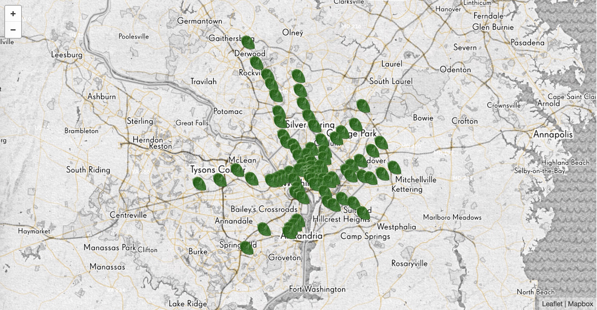
Exercise 05
Next Steps
Congratulations! You now have some hands-on experience geocoding using common Python data analysis libraries and working with one of the most popular Javascript web mapping libraries out there.
If you want to explore other web mapping features with Leaflet, there are a number of additional plugins to try out. Of particular interest may be ability to create time based visualizations and do heat-mapping.
Also, check out the Programming Historian Lesson Using Javascript to Create Maps of Correspondence that goes in depth on how to analyze correspondence using geospatial software, and using some of the same tools as this lesson.