
Contents
- Introduction
- Lesson Overview
- Learning Outcomes
- Suggested prior skills
- Lesson setup
- PDF conversion
- Fundamentals of Object Detection
- Processing the Images
- Identifying Smiles
- Download and Results
- Conclusions and next steps
- Endnotes
Introduction
Photographs are vital primary sources for modern historians. They allow later generations to ‘see’ the past — quite literally — in unique ways. Our understanding of the past two centuries would be poorer, and much less vivid, without these valuable sources.
Advances in Artificial Intelligence (AI) and Machine Learning (ML) – a branch of AI that uses computers to learn and gain knowledge from data without human supervision – raise the potential of asking new things from photographs, and of changing the role they play in the study of the past. In 2017, a group of researchers used a ML model known as a Convolutional Neural Network (CNN) to analyze almost 200,000 historical American high school yearbook photographs. They considered this an especially suitable test case for applying AI to the study of history. In their words, ‘yearbook portraits provide a consistent visual format through which one can examine changes in content from personal style choices to developing social norms.’1 Analyzing American yearbook photographs tracks the evolution of societal preferences throughout the 20th century, from what people wore in a formal photograph — glasses, neckties, earrings — to how they sat for a portrait — smiling or otherwise.
From police-operated surveillance cameras to facial recognition software at the airport, computer vision and ML — with their superhuman aptitude for pattern recognition — are becoming ubiquitous parts of many aspects of modern life. One of the historian’s tasks is to spot patterns in historical material, and ML’s ability to do this quickly over enormous amounts of data holds great potential. Even so, we must also critically examine the risks and biases inherent in applying systems designed for surveillance and security to the interpretation of the past, and there are serious ethical questions about the objectivity and reliability of these tools, as well as about whose perspectives are being prioritized or marginalized through their use (a topic that will be explored further in this lesson). Historians must approach AI and ML tools with a critical lens to maximize their utility while mitigating inherent biases.
Lesson Overview
This lesson is meant as an introductory exercise in applying computer vision ML to historical photos. The dataset we will explore contains several digitized American college yearbooks from the 20th century, now contained in Bethel University’s Digital Library. We have selected one yearbook per decade from 1911 to 1961. Certainly, many more yearbooks would yield more complete findings, but a limited dataset is sufficient for this exercise and will be processed much more quickly than a larger dataset. After extracting an individual image of each face, we will use a pre-trained library in Python called DeepFace to detect the presence of a smile in each photograph.
This test case will allow us to verify something easily spotted by traditional historical analyses: that early photographic portraits in the 20th century typically feature stoical, serious faces, while more recent photographs tend to feature more casual, smiling faces. Historians like Christina Kotchemidova, for example, have argued that early sitters for photos avoided smiling in order to appear more like subjects in painted portraits, and hence more dignified.2 The long exposure times of primitive cameras also discouraged posing with a smile. The proliferation of amateur photography in the 20th century led to less formal photography, and hence more smiling. This tutorial will allow us to test these assertions computationally.
This lesson will also serve as an introduction to some of the ethical issues posed by the use of AI in the study of photographs, particularly those implicating race and gender. ML image recognition can often miscategorize — or fail to identify entirely — non-white and female faces in photographs, a problem that can be compounded for historians by the simple fact that historical photographs are often of poor quality and low resolution. Indeed, ‘big data’ visual projects often use stable categories for their subjects, like ‘male’ or ‘female’, and faces are classified according to how closely they resemble other faces in either category. This can marginalize individuals who may not present as or identify with the categories used by the algorithm and researchers. Furthermore, historical photos often differ in theme, subject matter, and style from the contemporary photos which typically feature in ML training sets. Since there can be vast cultural differences between past and present, historical photos can thereby be misconstrued by modern aesthetic interpretations.
The makeup of the dataset used in this lesson presents further challenges from the standpoint of race and gender. Bethel University is a historically Christian institution that initially drew seminary students primarily of Swedish Baptist background from the upper Midwest of the United States. As the decades passed, and as Bethel became a four-year liberal arts college, its student body grew more diverse, but it remained majority male and white throughout the 20th century. While its yearbook collection adequately demonstrates the usefulness of applying ML principles to historical analysis, its homogeneous nature limits its value as a representational primary source. All of this is to say that applying a seemingly objective technological tool to the study of history is anything but objective. As with the other, more traditional tools in the historian’s bag, AI for facial recognition must be used with discernment.
Scholars from two broad perspectives may find this tutorial of interest. First, historians engaging with large visual corpora in their research, whether or not they’re specifically interested in facial recognition, may find computer vision generally and object recognition specifically valuable. Object recognition can allow one to track the changing frequencies of object presence in historical photographs over time. Or, more simply, object recognition can provide a technique for identifying photographs of interest in large visual collections for future close study.
Second, this tutorial is meant to provide an introductory lesson in how computational analysis of large visual collections can aid in curating and organizing large digital collections. In the conclusion, I suggest other pathways in computer vision that scholars may wish to pursue as next steps, including training their own model in object recognition. Of particular interest may be the two-part Programming Historian lesson Computer Vision for the Humanities: An Introduction to Deep Learning for Image Classification.
Learning Outcomes
At the end of the tutorial, you will be able to understand:
- The basics of computer vision machine learning
- How a computer ‘views’ an image
- How to extract pictures of human faces from historical documents digitized in the PDF format using Python, and how to organize them for further analysis
- How to apply a pre-trained computer vision model to a historical dataset
Suggested prior skills
You do not need to be a programming expert to complete this tutorial. To get the most out of it, however, you should have:
- Some knowledge of Python 3. Though this tutorial will not ask you to do any coding of your own, familiarity with how Python works will be beneficial
- A Google account, which will give you access to Google Colab where you can run the code yourself
- Basic familiarity with Google Colab and Jupyter notebooks. A Jupyter notebook is a document that contains code that you can run either directly online (i.e. without first setting up a programming environment on your computer) or on a local computer. A Google Colab notebook is a Jupyter notebook hosted on Google’s servers. For more, see the Programming Historian lesson on Jupyter notebooks.
Lesson setup
This lesson is accompanied by a Google Colab notebook which is ready to run. We have pre-loaded the sample dataset and all the code you’ll need. The Setting up Google Colab section will help you to orientate yourself within Colab if you’re new to the platform.
Alternatively, you can download the following files and run the code in your own Python environment:
- Bethel Yearbook 1911
- Bethel Yearbook 1921
- Bethel Yearbook 1931
- Bethel Yearbook 1941
- Bethel Yearbook 1951
- Bethel Yearbook 1961
- Python notebook
- An OpenCV pretrained facial detection model
haarcascade_frontal_default.xml
You should be aware that many ML processes require special configuration of your computing environment. For example, some of the packages below require both a C++ compiler, like Microsoft Visual Studio, and a capable dedicated graphics card (GPU). Both of these things are included in Google Colab, which can make it much easier to use than setting up your own machine learning environment, even for those with previous Python experience.
We will walk you through the necessary code step by step. Overall, it will:
- Download necessary files
- Convert each page of each yearbook to a
.pngimage - Pass what’s called a
haar cascadeover each image to identify a human face, and then save each found face as a separate.pngimage - Subject each face photo to a pre-trained object detector designed to identify smiles
- Produce a
.csvfile containing the ratio of smiling faces to non-smiling faces per year in the dataset
Setting Up Google Colab
If you’ve never used Google Colab before, you’ll want to familiarize yourself with how it works.
Click on the folder icon in the far left-hand column. This contains your virtual working environment. Think of it as Colab’s version of Windows Explorer or Finder on a Mac. As you progress through the notebook, you’ll see new folders and files appear here.
Next, Colab notebooks contain snippets of code called ‘cells.’ Each cell begins with a play button directly to the left of the first line of code. You’ll execute the code in this notebook by hitting each play button in order (you can let the previous cell finish executing before running the next one, or you can queue up the next cell while the previous one is running).
You can see the output of each cell directly below the code. As each cell runs, the play button will turn into a rotating circle and you’ll see a line at the very bottom of the screen that says ‘executing…’. When it has finished running, you’ll see a checkmark to the left of the cell as well as on the very bottom of the screen. You can then scroll down to run the next cell.
The first cell will create a folder in the left-hand panel called yearbook, which is where the necessary files will be downloaded. After the code runs, expand the dropdown next to the yearbook folder.
After you start the first cell, you should see:

Figure 1. Google Colab file hierarchy
You can double-click each PDF to download a copy if you wish to explore the scan of the original yearbook.
Preparing Your Environment
os.environ["CUDA_VISIBLE_DEVICES"] = "-1" allows the program to execute successfully. We're working on a permanent solution that continues to use the GPU as described in the lesson (September 2025).
Next, the code will install several Python libraries you’ll need later on. This step should take thirty seconds or so to build dependencies and download the necessary data. We will cover many of the installed and imported libraries in greater detail below. Note as well that the exclamation mark which appears before several lines is a special command in Colab, used to execute a bash command in a subshell. This code:
- Creates a working
yearbookfolder in the left panel, then downloads and unzips data from the hosted folder - Installs PyMuPDF, a PDF reader Python package, and machine learning libraries like OpenCV and DeepFace
- Imports various packages for further processing
%mkdir yearbook
%cd yearbook
!pip install --upgrade --no-cache-dir gdown
!gdown --id "1NHT8NN8ClBEnUC5VqkP3wr2KhyiIQzyU"
!unzip PHfiles.zip
%mkdir images
!pip install PyMuPDF
!pip install dlib
!pip install DeepFace
import os, shutil, fitz, cv2, numpy as np, pandas as pd, dlib, tensorflow as tf
from os.path import dirname, join
from deepface import DeepFace
os.environ["CUDA_VISIBLE_DEVICES"] = "-1"
PDF conversion
The next step accomplishes two things: first, it creates a separate folder for each yearbook. Then, it uses the Python library PyMuPDF to convert each yearbook .pdf file into individual .png image files, and saves them into the corresponding year folder.
Here is the full code you’ll need for this section. It will:
- Search for all files that end in
.pdf - Create a separate subdirectory in
/imagesfor each PDF and give it the same name as the PDF (e.g.,1911.pdfbecomes/images/1911) - Copy each PDF into its corresponding subdirectory
- Use PyMuPDF to open each PDF and convert each page to a
.pngfile
path = r'./'
pdfs = [f for f in os.listdir(path) if f.endswith('.pdf')]
for pdf in pdfs:
    os.chdir(os.path.join('./images'))
    os.mkdir((pdf.split(".")[0]))
    newdir = (os.path.join('./images/' + os.path.join(pdf.split(".")[0])))
    os.chdir("..")
    print ("Now copying images into " + (newdir))
    shutil.copy(pdf, newdir)
    os.chdir(newdir)
    doc = fitz.open(pdf)
    for page in doc:
      pix = page.get_pixmap()
      pix.save("page-%i.png" % page.number)
    os.chdir(os.path.dirname(os.getcwd()))
    os.chdir("..")
Most of the file organization steps in this tutorial use the Python os library. First you’ll specify the location of your folder and then create a list of the .pdf files using os.listdir:
pdfs = [f for f in os.listdir(path) if f.endswith('.pdf')]
Then, using a for loop, you’ll use os.chdir to move them into the /images subdirectory. The lines beginning with os.mkdir and newdir will create individual folders for every .pdf file. The code here will name each new folder based on the name of the .pdf file. For example, 1911.pdf will create a folder called 1911.
Next, the program will move into each new folder, copy the corresponding .pdf file into it, and use PyMuPDF to convert the .pdf file into separate .png images for each yearbook page. PyMuPDF (called with fitz in the code below) first opens the .pdf file, then uses a for loop to process the file:
for page in doc:
    pix = page.get_pixmap()
    pix.save("page-%i.png" % page.number)
For each page in the document, PyMuPDF will use the get_pixmap function to convert each page to a rectangular .png image. It then saves each image as a .png file giving it a name corresponding to its order in the original .pdf. When finished, you should see this file structure at the left:

Figure 2. Google Colab file hierarchy showing each yearbook page saved as a .png image
Fundamentals of Object Detection
Now that you have converted the yearbook PDFs to images, you can use the OpenCV ML library to search for and extract individual faces on each image. This process uses a machine learning approach called ‘object detection.’ To understand this approach, first, you need to understand the basics of computer vision, or how a computer ‘looks at’ an image.
Let’s take this image as an example:
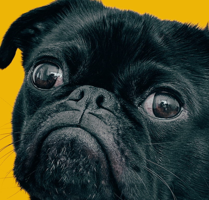
Figure 3. Image of a dog
If you zoom in, you can see that what human eyes perceive as an image of a dog are actually individualized, colorized pixels:

Figure 4. Zoomed in and pixelated image of dog’s nose
When a computer opens an RGB file such as a .png or a .jpg, each pixel is represented by three numbers, each between 0 and 255, which signify the intensities of that pixel in red, green, and blue. Higher values indicate more intense shades. For example, 0,0,255 indicates a pixel that is entirely blue. A .png or .jpg image with a resolution of 256x256 pixels therefore contains a list of 65,536 triple RGB color codes.
Displaying the image on your screen requires the software you’re using to convert the coded RGB values back to colorized pixels. The higher an image’s resolution, the larger the corresponding file, and the more computing power required to process it. Since computer vision processes typically deal with thousands of images, and usually many more, applications start by simplifying the image to allow the computer program to analyze its contents more quickly and with fewer resources. Often, the image resolution is downscaled significantly. Additionally, the three-digit RGB value can be converted to a single black/white intensity channel to further save resources, a process called ‘thresholding.’ You’ll see more examples of simplification below as we investigate how various computer vision techniques work.
How machine learning is used to recognize a particular object in a photo is more complex. Let’s start with a basic example, like a series of images of hand-drawn number eights. The parts of the images containing the number have different pixel color values than the negative space surrounding them. In supervised learning, the images that do contain the number 8 are assigned a value of 1 for ‘true’ (as opposed to 0 for ‘false’) by the human trainer. Given enough examples of images containing the number and feedback by the trainer, the computer will begin to recognize similarities in their RGB color values.
Once the computer has completed the training process, it is able to return a result predicting whether an image contains the pixel pattern which it has been trained to detect. This prediction is typically given in the form of a value between 0.00 and 1.00, with 1.00 representing probability that the computer has successfully detected the object in the image, and 0.00 the probability that it has failed to detect the image.
OpenCV and Haar Cascades
The particular kind of object detection library you’ll use in this lesson for facial recognition is called OpenCV, a computer vision library developed in the late 1990s. In particular, you’ll use a pre-trained face detection model in OpenCV called a Haar Cascade, which was developed by computer scientists Viola and Davis in 2001.3 Haar Cascades can reduce the computing power needed in object recognition because they don’t make calculations for each individual pixel, but rather look for pre-trained features, or patterns of groups of pixels throughout the image.
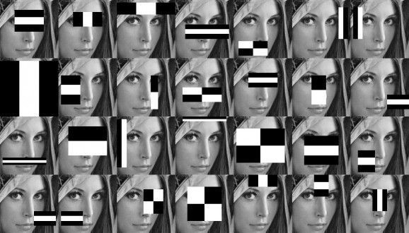
Figure 5. A Haar Cascade identifying pixel patterns on an image of a woman
In the rapidly changing modern ML landscape, OpenCV and Haar Cascades, both developed more than twenty years ago, represent older techniques. Researchers and practitioners of computer vision now often use more recent techniques called ‘deep learning,’ which we’ll get into in more detail below. Still, in part because they are an older, simpler, technology, it can be easier to understand the basics of image recognition using Haar Cascades than by jumping into more powerful modern algorithms. For this reason, you’ll test Haar Cascades out before turning to deep learning below.
Haar Cascades is also noteworthy for being flexible. By passing the object detector over many different sections of an image containing a human face, this method can recognize a face in any location in the image.
Figure 6. A Haar Cascade searching for pixel patterns in many sections of an image of a woman
This is particularly important for our purposes because the .png image of each yearbook page can contain many different human faces in different sorts of positions.
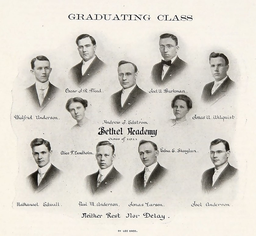
Figure 7. A page from the 1911 Bethel Academy yearbook featuring multiple people on a single page
Subjecting this image to a Haar Cascade, for example, results in several different detected faces (and one incorrectly identified face in a man’s necktie):
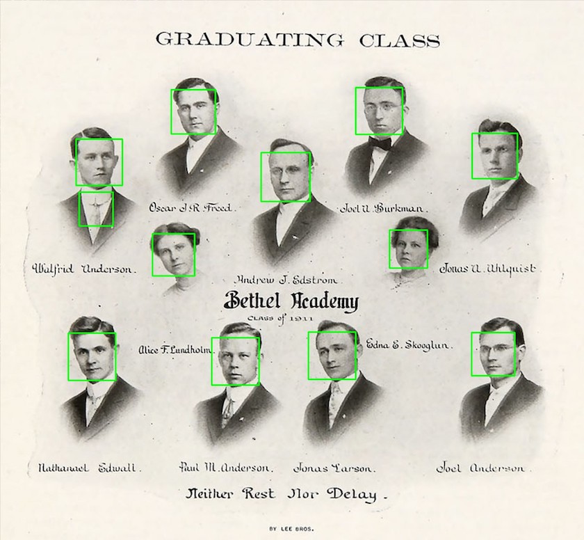
Figure 8. A page from the 1911 Bethel Academy yearbook featuring multiple people on a single page, with each face identified with a bounding box
Viola and Davis also developed an effective simplification technique for Haar Cascades, which allowed their model to identify faces very quickly and with a reasonably high degree of accuracy (around 95%). As the detector passes over the image a single time, areas which may contain a face are noted and identified as ‘weak classifiers.’ As more and more passes are made, if enough weak classifiers are detected in a certain area, they can rise above the specified threshold to indicate the presence of a face (and then become ‘strong classifiers’). This allows the Haar Cascade to focus only on areas of the image containing concentrations of weak classifiers, ignoring others and therefore saving resources and speeding up the process.
Finally, the lightweight, speedy nature of Haar Cascades means that this technique can be used by less powerful devices like laptops, cameras and smartphones, reducing or eliminating the need for powerful graphics cards required by many deep learning computer vision strategies. So, while many more recent ML computer vision models can exceed Haar Cascades in sheer power, Haar Cascades’ light weight and reasonably high accuracy have cemented their status in the modern computer vision toolkit.
Ethical Issues with Facial Recognition
Now that you’ve explored how computer vision typically relies on differences in pixel color density, you can begin to recognize some of the ethical dangers of using this technology when it comes to skin color. Simply put, photographs of lighter skin tones often contain greater differences in pixel density than darker skin tones, which means that some algorithms can fail to detect or misidentify people with darker skins. The sample historical dataset, in which darker skins are underrepresented, makes the issue even more challenging.
The early decades of Bethel University’s yearbook contain photos of predominantly white, male faces. Failing to identify the few minority students in early yearbooks only further suppresses representation of communities long disadvantaged in American higher education. The Algorithmic Justice League has shown that the misidentification of darker skinned people can play a crucial role in promoting racial bias and discrimination.
Here is an example of the computer failing to recognize a non-white face from the dataset:
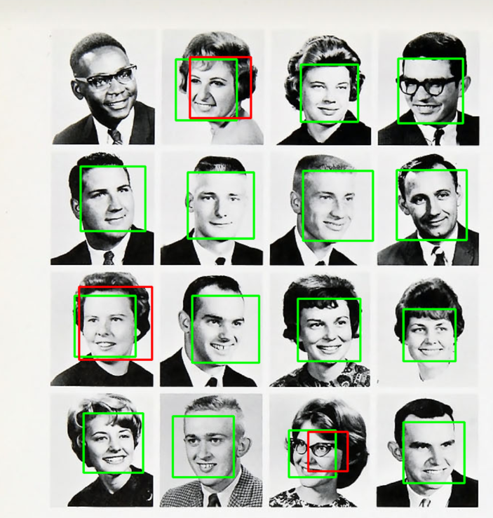
Figure 9. A page from the Bethel College yearbook in the 1960s featuring multiple people on a single page. The computer vision tool has correctly identified fifteen White faces, but failed to identify the face of the sole Black male in the photo.
Bethel’s historically majority White student body is sure to impact the nature of our dataset, and hence our findings. For example, Wondergem and Friedlmeier have found that African American males historically smiled less frequently in American high school yearbooks from predominantly Black schools than from predominantly White schools.4 Such details make extrapolating larger conclusions from our limited dataset difficult, though its suitability as a test case for ML and computer vision principles remains sound once its idiosyncratic nature is recognized.
Research in facial recognition has confirmed that algorithms still tend to be most inaccurate when assessing faces with darker skin tones, female features, or in the 18-30 year-old range. The 2018 AI project, Gender Shades, found that the error rate for young, darker skinned women in particular was 34% higher than for lighter skinned men in one study.5 As more and more police departments turn to facial recognition for surveillance, the moral weight of such bias in computer vision should be obvious.
The issue of bias in computer vision software is also of acute importance for historians, since historical photographs may have been taken with primitive cameras, may have faded and lost contrast over time, and/or may have been scanned and rescanned many times. All of these factors can exacerbate the biases already inherent in current facial detection and recognition processes.
Still, there are several solutions that can promote a more ethical application of computer vision technology. Most importantly, the training data that AI companies have used to develop facial recognition software has traditionally been overwhelmingly dominated by images of White men.6 Discrepancies in facial recognition by race and gender can therefore be greatly reduced diversifying the training data. Additionally, as camera technologies continue to improve along with artificial intelligence techniques, photographs of darker skinned people should be more easily identified by AI algorithms. Fine tuning pre-trained models that have been shown to be biased can also help. For groups traditionally underrepresented in historical photographic datasets, like women and non-white people, Wang and Russakovsky have found that increasing the proportion of photographs of them when fine-tuning the dataset can improve the model’s performance in recognizing these groups and therefore reduce bias.7
Finally, overly simplistic classification schemes - researchers often use ‘Caucasian’/’White’, ‘Asian’, ‘African’/’Black’ and ‘Indian’ as the sole racial or ethnic classifiers — should be replaced with more specific categories, which again would require broader, more representative training data.8 A more complex labeling scheme, however, would also require greater discretion from those doing the labeling, and could itself lead to additional ethical concerns (especially if the annotators are not also diverse).
Processing the Images
Now that you’ve prepared your dataset, and considered the methodological and ethical issues involved with object detection for facial recognition, you can proceed with processing the PNGs for facial recognition, while also ensuring that the output is clearly organized for future steps.
Here is the full code you’ll need for this section. It will:
- Move to the
/imagessubdirectory and walk through all folders looking for files that end in.png - Create a subdirectory called
/YEAR faces(e.g./1911 faces) - Use OpenCV (here
cv2) to:- Convert each image to greyscale (this reduces the computing power necessary to analyze each image)
- Pass a haar cascade identifier (
haarcascade_frontalface_default.xml) over each image looking for facial features x,y,w,hrefer to pixel locations that OpenCV uses to denote where the human face occurs on the image. The script adds a few pixels of padding on top of this, so the face does not extend to the edge of the image.- If it identifies a human face, it will save it as a
.pngimage and places it in the/YEAR facessubfolder - Use a
try/exceptloop to continue the code if an error occurs
path = r'./'

os.chdir(os.path.join(path + 'images'))
dirs = os.listdir(path)
for dir in dirs:
    os.chdir(os.path.join(path + dir))
    pngs = [f for f in os.listdir(path) if f.endswith('.png')]

    if not os.path.exists((dir) + ' faces'):
        print("New 'faces' directory created in " + (dir) + " folder")
        os.makedirs((dir) + ' faces')

        count = 0
        for png in pngs:
            image = cv2.imread(png)

            greyscale_image = cv2.cvtColor(image, cv2.COLOR_BGR2GRAY)

            face_cascade = cv2.CascadeClassifier(cv2.data.haarcascades + "haarcascade_frontalface_default.xml")

            detected_faces = face_cascade.detectMultiScale(image=greyscale_image, scaleFactor=1.9, minNeighbors=4)

            count = 0
            for (x,y,w,h) in detected_faces:
                try:
                    xpadding = 20
                    ypadding = 40
                    crop_face = image[y-ypadding: y + h+ypadding, x-xpadding: x + w+xpadding]
                    count+=1
                    face = cv2.rectangle(crop_face,(x,y),(x+w,y+h),(255,0,0),2)
                    cv2.imwrite(path + (dir) + ' faces/' + str(count) + '_' + png, face)
                except (Exception):
                    print("An error happened")
                    continue
            os.remove(os.path.join(path, png))
    os.chdir("..")
The first step in the code simply identifies your root folder and creates a variable (dirs) containing a list of all of the subfolders within it. Next, you use a for loop to change directories into each subfolder and create another list with every file in that subfolder that ends in .png:
os.chdir(os.path.join(path + 'images'))
dirs = os.listdir(path)
for dir in dirs:
    os.chdir(os.path.join(path + dir))
    pngs = [f for f in os.listdir(path) if f.endswith('.png')]
In the next step, you create a new folder with the format /YEAR faces (so, /1911 faces and so on):
    if not os.path.exists((dir) + ' faces'):
        print("New 'faces' directory created in " + (dir) + " folder")
        os.makedirs((dir) + ' faces')
The steps that follow get into the meat of facial recognition. With another for loop, you open each .png file with OpenCV (cv2 in the code), a robust set of Python libraries for computer vision and machine learning. Some of the later yearbooks contain color pictures, so we simplify the file by converting each image to greyscale (since greyscale images are faster to process than color), and pass over it a Haar Cascade classifier specifically trained by OpenCV to detect human faces.
The two adjustable parameters in face_cascade.detectMultiScale are scaleFactor and minNeighbors. The first refers to how significantly the image is downscaled before processing (larger numbers mean more downscaling and less data), and the latter refers to the confidence level required for the program to classify something as a face (higher is more rigorous but may miss some faces).
for png in pngs:
    image = cv2.imread(png)
    greyscale_image = cv2.cvtColor(image, cv2.COLOR_BGR2GRAY)
    face_cascade = cv2.CascadeClassifier(cv2.data.haarcascades + "haarcascade_frontalface_default.xml")
    detected_faces = face_cascade.detectMultiScale(image=greyscale_image, scaleFactor=1.9, minNeighbors=4)
The final for loop in this cell determines how large the new .png image containing each face should be. x, y, w, and h all refer to pixel locations for corners of a bounding box drawn on each recognized face. The try loop adds some additional pixels to this box as a cushion, and then crops the image. Finally, the resulting image is saved to a new .png file in the /YEAR faces folder.
for (x,y,w,h) in detected_faces:
                try:
                    xpadding = 20
                    ypadding = 40
                    crop_face = image[y-ypadding: y + h+ypadding, x-xpadding: x + w+xpadding]
                    count+=1
                    face = cv2.rectangle(crop_face,(x,y),(x+w,y+h),(255,0,0),2)
                    cv2.imwrite(path + (dir) + ' faces/' + str(count) + '_' + png, face)
                except (Exception):
                    print("An error happened")
                    continue
            os.remove(os.path.join(path, png))
Identifying Smiles
In the final intensive step, where we identify which photos contain smiling faces and which ones don’t, you’ll use a more sophisticated kind of machine learning process called a Convolutional Neural Network (CNN). Haar Cascades were suitably lightweight and fast enough for an exploratory first step, but they aren’t the best for recognizing features that deviate from those they’ve been trained to recognize. For example, if you didn’t include photos of a person wearing false glasses and a top hat in your training data, a Haar Cascade might not recognize such an image as containing a human face.
In the decades since the Haar Cascades technique was developed in 2001, huge advances in AI have taken place that allow for finer distinctions in object recognition, particularly those situations that involve the algorithm evaluating images without a human instructor, otherwise known as ‘unsupervised’ learning (though most object detection methods still require initial supervision to identify what objects should be detected). These more modern algorithms harness the power of recently developed GPUs to look for dozens and dozens of distinct patterns within an image, most of which the computer ‘learns’ simply by viewing similar images and correcting its own mistakes in prediction.
In AI terminology, each individual pattern in the CNN is called a ‘neuron.’ Simplistically, one neuron might be dedicated to recognizing the pixel patterns at the corner of a left eye, another to the bottom of an ear lobe, etc. When the computer evaluates a photo looking for a smiling human face, these individual neurons pass their evaluations and predictions to the next series of calculations (typically called the next ‘layer’ within the CNN), which contain more neurons that take the previous layer’s calculations into account and look for yet more patterns, before passing the updated information on to the next layer, and so on. This kind of multi-faceted detection program is an example of deep learning because the algorithm continually refines its evaluation through multiple layers. Through a refinement process commonly known as ‘backpropagation,’ the CNN compares its predictions with the correct answers, and adjusts the connections between the neurons accordingly, thereby improving the results. Like Haar Cascades, CNNs are capable of detecting objects anywhere in the image as it passes (or ‘convolves’) the detector over various stages of the image.
The particular deep learning library you’ll use here is called DeepFace, which comes with several pre-trained models that can be used to detect and classify various categories in images of human faces, like age, gender, emotion, and race. Given the current ethical state of AI in regards to race and gender, which we discussed above, we’ll limit the experiment to DeepFace’s emotion classifier. For our purposes, we’ll say that a photo designated as ‘happy’ contains a smile, while a photo with any other dominant emotion, or a photo lacking any dominant emotion, does not. We should note here that even emotion detection algorithms are not inherently objective, as the facial cues for human emotions are not themselves universal.
In the code below, you’ll create a series of counts for each year that tallies the number of times the object detector classifies images as containing either smiles or non-smiles. It will then compare these counts against a count of total images, which will allow us to calculate a ratio of smiles to non-smiles for any given yearbook edition:
%cd ..
number_smiles = 0
smile_counts = []
number_nonsmiles = 0
nonsmile_counts = []
num_errors = 0
error_counts = []
pngs = []

file_count = 0
file_count_list = []

years = ['1911', '1921', '1931', '1941', '1951', '1961']

for year in years:
    path = r'./images' + '/' + year
    for root, dirs, files in os.walk(path):
        for _ in dirs:
            path = path + '/' + (year + ' faces')
            if(file_count != 0):
                file_count_list.append(file_count)
            file_count = 0
            for f in os.listdir(path):
                if f.endswith('.png'):
                    pngs.append(path + '/' + f)
                    file_count = file_count + 1
The part of the cell that analyzes faces for smiles is yet another for loop:
for png in pngs:
    try:
        total_loops = total_loops + 1
        count = count + 1
        if(count != (file_count_list[iterator] + 1)):
            demography = DeepFace.analyze(png, actions = ['emotion'])
            print(demography)
            if(demography[0]['dominant_emotion'] == 'happy'):
                number_smiles = number_smiles + 1
            else:
                number_nonsmiles = number_nonsmiles + 1
        else:
            count = count - 1
            smile_counts.append(number_smiles / count)
            nonsmile_counts.append(number_nonsmiles / count)
            error_counts.append(num_errors / count)
            number_smiles = 0
            number_nonsmiles = 0
            num_errors = 0
            iterator = iterator + 1
            count = 0
If the DeepFace.analyze function classifies the photo as containing a face with the dominant ‘happy’ emotion, the program will add 1 to the number_smiles list. If the module detects any other emotion, or is unable to return a confident prediction of the emotion presented in the photo, it will update the count in either the number_nonsmiles list or the num_errors list.
Finally, the program will take these three numbers (four if we include the count for total images) and create a Pandas dataframe, saving it as a .csv file:
smile_counts.append(number_smiles / count)
nonsmile_counts.append(number_nonsmiles / count)
error_counts.append(num_errors / count)

header = {'Years': years, 'Smiles': smile_counts, 'Non-Smiles': nonsmile_counts, "Error Weight": error_counts}
data = pd.DataFrame(header)
data.to_csv('YearbookOutput.csv', index=False)
Download and Results
The final step involves downloading the .csv file. Run the code below:
from google.colab import files
files.download('YearbookOutput.csv')
You can also click the three dots to the right of the YearbookOutput.csv file to the left of the Google Colab notebook and select Download. Once you’ve opened the downloaded file in a spreadsheet software, you can explore the results.
How did we do? As you can see, the smile detector found an overall increased rate of smiles in the dataset as the 20th century progressed. (Your .csv file will probably look different to ours, as slightly different results are expected each time the program runs.) The first two yearbooks, from 1911 and 1921, contain no smiling faces. The 1931 yearbook features smiles at a rate of about 15%, 1951 at about 25%, and 1961 at about 43%. The outlier in this otherwise steady progression is the yearbook of 1941, which features only about 3% smiling faces. A closer look at this particular yearbook reveals that it has relatively few photos where students sat for individual portraits; larger group shots and more casual pictures of campus life dominate. These different photo settings might have influenced the final results; or perhaps the photographer instructed students not to smile during group shots. Either way, this anomalous yearbook is a good reminder of the importance of favoring large datasets for this type of analysis, as one outlier can skew the overall results within smaller sets like ours.
If we draw some qualitative conclusions from this small sample dataset, 1961 is the first year where smiles began to rival non-smiles in total numbers. Claudia Goldin and Lawrence F. Katz have argued that while American higher education gradually became more and more coed (mixed genders) from the mid-1800s to the mid-1900s, the switch from single-sex to coed education accelerated rapidly in the 1960s and 1970s.9 The greater share of smiling faces in yearbooks from the 1960s might be a part of other, wider social changes in the American collegiate landscape. Further analysis of this data by sorting faces based on gender would be needed to confirm whether Bethel’s student body became markedly more female in these years, but of course that process would be fraught by the ethical challenges of gender-based facial recognition described above.
Let’s continue our analysis and zero in on the Error Weight column of the .csv file:
| A | B | C | D | |
|---|---|---|---|---|
| 1 | Years | Smiles | NonSmiles | Error Weight |
| 2 | 1911 | 0 | 1 | 0 |
| 3 | 1921 | 0 | 0.923076923 | 0.076923 |
| 4 | 1931 | 0 | 0.7 | 0.3 |
| 5 | 1941 | 0.066666667 | 0.4 | 0.533333 |
| 6 | 1951 | 0.171929825 | 0.684210526 | 0.14386 |
| 7 | 1961 | 0.385964912 | 0.526315789 | 0.087719 |
Error Weight contains the frequency that the smile detector failed. Dlib, the sub-library of DeepFace we used to identify smiles, promises accuracy of up to 99.38% in some contexts. As you can see, our results were not as accurate, though we did approach the upper 90th percentile in the later decades.
This would confirm the common sense hypothesis that computer vision techniques will be less accurate when applied to older photographs. It also underscores the importance of the historian maintaining familiarity with their dataset, even a large one subjected to machine learning. Even so, an error rate in the low single digits for photographs after the mid-twentieth century should give researchers confidence in using ML on large visual corpora.
If you’d like to run the experiment on a larger set of yearbooks, you can browse more Bethel Yearbooks in their Digital Library.
Conclusions and next steps
This lesson has provided an introduction to the computer vision technique of object recognition, using the increased frequency of smiles in 20th century yearbook photographs as a test case. Detecting the presence of smiles in a visual database is indeed a very specific task that most historians will not find particularly applicable. Still, using ML to identify patterns and trends in large visual collections holds great promise for streamlining and simplifying important tasks in historical research, as well as for turning historical collections into data. For example, crowd-sourcing projects like Freedom on the Move and many of the humanities-based projects on the crowd sourcing site Zooniverse have leveraged human input for some of the repetitive tasks which historians and curators face in managing large collections, such as identifying and labeling metadata. Computer vision and object recognition promises to greatly hasten such efforts, reducing or perhaps even eliminating much of the tedious human labor required.
In regards to large visual corpora in particular, the use of computer vision strategies can help further what Taylor Arnold and Lauren Tilton call ‘distant viewing,’ a parallel to the common Digital Humanities application of ‘distant reading’ techniques used in the study of large textual corpora.10 Computer vision and object recognition can help scholars bridge what is often called the ‘semantic gap’ between the information contained in a photograph or image and the cultural meaning which humans derive from it. By specifying aspects or characteristics of image collections that contain historical meaning, and then training machine learning algorithms to search for them — whether it’s a smile, fashion choice, use of a particular object, or something else — researchers can add ‘a new layer of meaning to the raw pixels’ contained in the images, and then apply such insights quickly at large scales.11 Similar to the contrasts inherent in distant vs. close reading in digital literary studies, distant viewing of images and photographs can complement and support conclusions gleaned from closer, more traditionally humanistic examinations.12
One benefit of introducing computer vision with a simple experiment like smile recognition is that it makes possible the use of pre-trained facial recognition models like OpenCV’s Haar Cascade and DeepFace’s emotion identification. While there are other pre-trained open source object recognition models available online, like Google’s Open Images database, scholars interested in using object recognition in their own work may find it necessary to train their own model, or adapt a pre-existing one using deep learning. The learning curve for developing your own model can be high, though the two-part Programming Historian tutorial Computer Vision for the Humanities: An Introduction to Deep Learning for Image Classification, provides thorough instructions for this approach, tailor-made for historians and other humanists. Hugging Face also maintains a list of pre-trained object detection models.
Additionally, there are several companies like Roboflow which offer hosted computer vision trainers with a point-and-click graphical user interface. The trained model can then be downloaded and integrated into an object detector and executed with Python, as in this lesson. However, even if professional companies offer heavily discounted educational licenses, there can still be financial costs. Furthermore, many of these proprietary softwares may require researchers’ data to made public, or at the very least to be made available to the cloud-hosting company.
Endnotes
-
Shiry Ginosar, Kate Rakelly, Sarah M. Sachs, Brian Yin, Crystal Lee, Philipp Krähenbühl and Alexei A. Efros, “A Century of Portraits: A Visual Historical Record of American High School Yearbooks,” IEEE Transactions on Computational Imaging, 3 no. 1 (September 2017): 1, https://arxiv.org/pdf/1511.02575.pdf. ↩
-
Christina Kotchemidova, Why We Say “Cheese”: Producing the Smile in Snapshot Photography,” Critical Studies in Media Communication, 22 no. 1 (2005): 2-25, https://www.tandfonline.com/doi/abs/10.1080/0739318042000331853. ↩
-
Paul Viola and Michael Jones, “Rapid object detection using a boosted cascade of simple features,” Proceedings of the 2001 IEEE Computer Society Conference on Computer Vision and Pattern Recognition, CVPR 2001 (2001): 1-9, https://ieeexplore.ieee.org/document/990517/authors#authors. ↩
-
Taylor R. Wondergem and Mihaela Friedlmeier, “Gender and Ethnic Differences in Smiling: A Yearbook Photographs Analysis from Kindergarten Through 12th Grade,” Sex Roles 67, no. 7-8 (2012): 403-411. https://doi.org/10.1007/s11199-012-0158-y ↩
-
Joy Buolamwini and Timnit Gebru, “Gender Shades: Intersectional Accuracy Disparities in Commercial Gender Classification,” Proceedings of Machine Learning Research, 81 (2018): 1–15, http://proceedings.mlr.press/v81/buolamwini18a/buolamwini18a.pdf. ↩
-
Hu Han and Anil K. Jain, “Age, Gender and Race Estimation from Unconstrained Face Images,” (2014) http://biometrics.cse.msu.edu/Publications/Face/HanJain_UnconstrainedAgeGenderRaceEstimation_MSUTechReport2014.pdf. ↩
-
Angela Wang and Olga Russakovsky, “Overwriting Pretrained Bias with Finetuning Data,” 2023 IEEE/CVF International Conference on Computer Vision (ICCV), Paris, France (2023): 3934-3945, https://openaccess.thecvf.com/content/ICCV2023/papers/Wang_Overwriting_Pretrained_Bias_with_Finetuning_Data_ICCV_2023_paper.pdf. ↩
-
Mei Wang, Weihong Deng, et al., “Racial Faces in-the-Wild: Reducing Racial Bias by Information Maximization Adaptation Network,” Proceedings of the 2019 IEEE Computer Society Conference on Computer Vision and Pattern Recognition, CVPR 2019 (2019): 692-702, https://arxiv.org/pdf/1812.00194.pdf. ↩
-
Claudia Goldin and Lawrence F. Katz, “Putting the “Co” in Education: Timing, Reasons, and Consequences of College Coeducation from 1835 to the Present,” Journal of Human Capital, 5 no. 4 (2011): 377-417. ↩
-
Taylor Arnold and Lauren Tilton, “Distant viewing: analyzing large visual corpora,” Digital Scholarship in the Humanities (2019): 1-14, https://www.distantviewing.org/pdf/distant-viewing.pdf. ↩
-
Ibid. 3. ↩
-
See also Tuomo Hiipala, “Distant viewing and multimodality theory: Prospects and challenges,” Multimodality and Society, 1 no. 2 (2021), 134-52, https://journals.sagepub.com/doi/pdf/10.1177/26349795211007094. ↩