
Contents
- Introduction
- Lesson Aims
- Historical Background and Data
- Setting up your Coding Environment and Creating the Shiny Application
- Coding the Application
- Creating the Server Logic
- Improving the Application
- Conclusion
- Final code
- End Notes
Introduction
This lesson demonstrates how to build a basic interactive web application using Shiny. Shiny is a library (a set of additional functions) for the programming language R. Its purpose is to facilitate the development of web applications, which allow a user to interact with R code using User Interface (UI) elements in a web browser, such as sliders, drop-down menus, and so forth. In the lesson, you will design and implement a simple application, consisting of a slider which allows a user to select a date range, which will then trigger some code in R, and display a set of corresponding points on an interactive map.
Lesson Aims
In this lesson, you will learn:
- How to create a basic interactive Shiny application.
- The key layouts and design principles of the Shiny UI.
- The concept and practice of ‘reactive programming’, as implemented by Shiny applications. Specifically, you’ll learn how you can use Shiny to ‘listen’ for certain inputs, and how they are connected to outputs displayed in your app.
Graphical User Interfaces and the Digital Humanities
Graphical User Interfaces (GUI) and interactive elements can help to make certain types of data-driven scholarly work more accessible or readable. To give a simple example, historians working with large-scale data might want to demonstrate the change in a variable over time. An interactive map with an adjustable timeline is, in some cases, easier to read and allows for more granularity than a series of static maps. Allowing a user to set the parameters of the visualisation can help to avoid some of the bias often found in data visualisations using time series (for example, arbitrarily drawing one map per decade).
Many research projects have interactive elements as outputs. Some examples include the Tudor Networks of Power visualisation of the networks in the Tudor State Papers, the interactive Press Tracer, and (to give an example using Shiny), the GeoNewsMiner, which displays geocoded place-mentions in a corpus of newspapers. Interactive applications can also be useful tools for archivists: researchers at the National Archives UK have created an app using Shiny which assesses the risk level in a digital collection through a series of questions answered by a user.
Another typical use-case for interactive applications is to provide an easier way to explore your own dataset, without ever intending for the application itself to be made publicly available. One might simply use interactive data visualizations to find interesting patterns or as a starting point for further research. In this way, interactivity can be particularly useful in helping explore and find patterns within large-scale datasets.
Options for creating a GUI
There are a number of ways one could approach the development of interactive visualisations similar to the examples above. One is to learn a specialist tool designed for manipulating web pages in response to data inputs, such as the Javascript library D3. A second option would be to use existing web-based tools, either general ones such as Tableau and Rawgraphs, or ones with a more specific purpose such as Palladio or Gephi. A third approach might be to use Jupyter notebooks, which allow you to share interactive code, and even, with some additional packages, to create a user interface.
This lesson covers a fourth approach: making interactive applications with a GUI using a library for a general-purpose programming language, such as Bokeh or Dash for Python, or, as used in this tutorial, Shiny for R. Both Python and R are open source, widely-used, versatile programming languages, with active communities and a huge range of third-party packages. There are many circumstances where it makes sense to use these as the basis for interactive applications. In essence, these packages act as interactive interfaces to the programming language, allowing for the creation of sliders, selectors, and so forth, which can then be used as inputs to dynamically change bits of code. In most cases, they require no technical expertise from the end-user. As they are designed to work in a browser, they work on any platform, and are easy to share.
Shiny and Reactive Programming
Shiny is based around a concept called reactivity. Usually, when coding, we set a variable to a specific value, say x = 5. In reactive programming, the variable is dependent on a changing input, usually set by a user (from a text slider or drop down list, for example). The code ‘listens’ for changes to these reactive variables and every time these special variables change, any output they are used to generate automatically updates.
However, this updating only happens within reactive contexts. Shiny has three important reactive contexts: render* functions, which are used to create R objects and display them in the app, observe({}), and reactive({}). In this tutorial you’ll use reactivity to create a summarised dataframe of newspaper titles and their dates, which updates dynamically based on a user input of dates. Elsewhere in your app, you’ll use a render* function to display a map which will listen for changes to this reactive dataframe and update itself when any is found.
Advantages and Disadvantages of Using Shiny
The advantage to this approach is that creating Shiny applications is relatively simple if you already know R, and R’s entire range of libraries and features can be harnessed by Shiny. In some circumstances, this might be preferable to learning a new language from scratch. If you have experience with R and just a little knowledge of Shiny, you can create very complex and useful applications, covering everything from maps to network analysis, from machine learning models to full dashboards with lots of functionality. If you can program it with R, you can probably make it interactive with Shiny. The process of creating a Shiny UI is very flexible and easy to customise, meaning it is straightforward to make an application in a format that could be embedded into a project website using iframes: see the Mapping the Gay Guides project for one example.
There are some drawbacks worth considering. For those who have no intention of using a language like R in other aspects of their work, learning it just to produce Shiny apps may be overkill. Shiny is open source and free to use, but by far the easiest way to publish your finished application to the web is using a service called shinyapps.io. Shinyapps.io is a commercial product with a free tier giving a limited number of hours of use (25), and after that you’ll need to pay a monthly fee. You can run Shiny on your own server (or through something like Amazon Web Services), but it’s quite an involved process and requires some pretty advanced knowledge of configuring web servers. You should bear this in mind if you are thinking about using Shiny for a public-facing output, particularly if you think it might have lots of traffic and heavy use. As an alternative, some of the functionality of Shiny can be replicated in a simple HTML page using the R package crosstalk.
Historical Background and Data
The national library of the United Kingdom, the British Library, holds by far the largest collection of British and Irish newspapers in the world. The earliest serial news publication in its collection is from 1621, and it continues to collect to this day. The Library’s catalogue holds a wealth of information on its newspaper holdings, which has been made publically available in the form of structured metadata. This metadata is essentially a list of newspaper titles, containing the publication dates and places, title changes and merges, and information on microfilm surrogates and digital holdings.
This structured metadata is the resource which you will use in this lesson. Tracing the metadata of this collection is a way for historians to chart the growth and change in the press over time and through different regions. Furthermore, it may help us to understand more about the Library’s collection itself, including its gaps, biases, digitisation strategies and blind spots. The data might even indicate something about the changing demographics and industrialisation of Britain, as well as developments in communication technologies (trains and then telegraphs made it possible to have regional and local presses, for instance).
The newspaper industry (and therefore the collection) grew from a tiny number of titles published in London in the early seventeenth century to a flourishing weekly and daily provincial press in the eighteenth, and then a very large local press in the nineteenth and twentieth centuries. For much of the eighteenth century, a tax was added to every copy of a newspaper making them expensive and only available to the elite. In the following century this was repealed, and the press began —albeit slowly— to reflect the aspirations and diversity of the country and its various regions more fully. The application you’ll create in this tutorial —an interactive map of published titles, controlled by a user-selected time slider— is a useful way to visualise these changes.
Getting Hold of the Data
For this tutorial you will need to download two files: first, a title-level list of British and Irish newspapers (which will be referred to as the ‘title list’) and second, a helper dataset of place names and coordinates (which we’ll refer to as the ‘coordinates list’) for matching the places found in the title list to locations on a map.
1. To get the title list, visit the British Library repository. The list is available on the repository in two formats: either a .zip file containing a .csv and a readme, or as an Excel spreadsheet. For this lesson, we’ll work with the .csv format. Download the .zip file, and unzip it. Alternatively, you can download a copy of the dataset used in this tutorial on Github. To download this file, just view the raw version and save the page locally.
2. The coordinates list is also available on Github. To download this file of coordinates, just view the raw version and likewise save the page locally.
Understanding the Title List
Once this is done, take a look at the title list dataset (you can open it in R, a spreadsheet program or a text editor). The title list has been produced by the British Library and is published on their institutional repository. It contains metadata taken from the Library’s catalogue of every newspaper published in Britain and Ireland up until the year 2019, a total of about 24,000 titles. There is more information available in a published data paper.1
The .csv file (BritishAndIrishNewspapersTitleList_20191118.csv) contains a number of fields for each title, including the name of the publication, subsequent and previous title names, several fields for geographic coverage, the first and last dates held, and some other information.
It’s worth reading the README file which comes along with the .zip file. This explains that there are several fields provided for geographic coverage, because the records have been catalogued over a long period of time, during which cataloguing standards and conventions have changed. The purpose here is to map the newspapers at a geographic point level, i.e., at the level of village, town, or city, rather than county or country. There are two fields where we might find the relevant geographic points to map: place_of_publication and coverage_city. These seem like different things (a newspaper could be published in one place but have geographic coverage over another, perhaps if the former didn’t have a suitable newspaper press), but that’s not how they’ve been used by cataloguers in practice. The README file says that the latter (coverage_city) contains more complete data, so that is the one you’ll use to map the titles.
The other two fields of interest are the first and last dates held. The readme also tells us that the library does not have complete coverage, though it has most titles from the 1840s onwards, and effectively all titles from 1869 when Legal Deposit2 was introduced. This means that the collection does not necessarily have all issues of a newspaper between the first and last dates held by the Library.
In this tutorial, you’ll create an interactive slider which will allow a user to choose a start and an end date. This could be used to filter the data in one of two ways: either to show every newspaper published at some point between those two dates, or to map every newspaper first published between two given dates. Because the former scenario it would over-represent the Library’s collections, to keep things simple, in this tutorial you’ll work on the latter visualization of every newspaper published within a certain time frame.
Setting up your Coding Environment and Creating the Shiny Application
To demonstrate how Shiny works, in this tutorial you will take this dataset of newspaper titles, places of publication, and dates, and turn it into a basic interactive application. In total there are five short coding tasks your application will need to carry out:
- Load the two necessary datasets
- Create a user interface
- Create a ‘reactive’ dataset of places, a count of their appearances, and their geographic coordinates
- Turn this ‘reactive’ dataset into a special geographic dataset, called a simple features object
- Create an interactive map using the R library, Leaflet
First, however, you need to set up the correct programming environment and create a new Shiny application.
Install R and Rstudio
To get started with this tutorial, you should install the latest versions of R and Rstudio on your local machine. The R programming language has a very popular IDE (Integrated Development Environment) called RStudio, which is often used alongside R, as it provides a large set of features to make coding in the language more convenient. We’ll use RStudio throughout the lesson.
Previous Programming Historian lessons have covered working with R and working with the tidyverse. It would be useful to go through these lessons beforehand, to learn the basics of installing R and using the tidyverse for data wrangling.
Create a new RStudio Project
Once you have a working copy of R and Rstudio, open RStudio and create a new project to develop your application. Open the ‘Create a Project’ dialogue window using the menus (File->New Project). Select ‘New Directory’, then ‘New Project’. Name your project directory and press ‘Create Project’.
Before you continue, install the four packages necessary to complete the tutorial, if you don’t have them already. Three of these can be installed directly through R Studio; the fourth might require extra steps. In the R console or in a separate R script, run the following commands:
install.packages('shiny')
install.packages('leaflet')
install.packages('tidyverse')
install.packages('sf')
Depending on your system setup, the fourth package, sf, may require additional steps before it can be installed. Windows users should be able to install directly using install.packages('sf'), but Mac users may need to install a third-party library, gdal, before the installation will work, using Homebrew. Install gdal by opening a Terminal window and entering the following commands:
brew install pkg-config
brew install gdal
The latest instructions and further details can be found on the package Github page, including instructions for various Linux distros. Check the instructions under the Installing header in the linked Github Readme file.
Create an Empty Shiny Application
A Shiny application consists of a script file with a special, reserved filename, app.R, which tells R Studio to treat that script as an application and open it in a web browser when it is run. In this first section, you will create an application which will load the relevant libraries and datasets, and display a test ‘Hello World’ message. To do this, carry out the following steps:
1. Set up an Application Folder
It’s good practice to put all the necessary files for the application in their own folder, within the RStudio project. Do this by creating a new folder called ‘newspaper-app’ within the folder of the RStudio project you just created. Place the files you downloaded above (BritishAndIrishNewspapersTitleList_20191118.csv and newspaper_coordinates.csv) into this new folder.
2. Make the app.R file.
With RStudio open, click File-> New file -> R Script. Use the menu or command/ctrl + s to save the file. Navigate to the new folder you’ve just created, and save the file there, entering app.R as the file name. You should now have the following files in the ‘newspaper-app’ folder you just created:
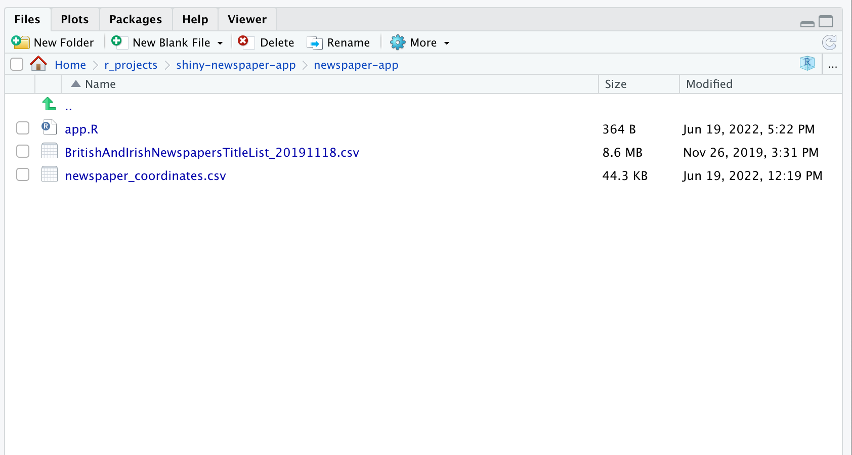
Figure 1. Screenshot of application folder showing the files needed.
3. Load the relevant libraries
The first thing the app will need to do is prepare and load the data. This is done within the app.R script, but outside the UI and server elements you’ll create in a moment. First, load all the libraries you need to use by entering the following into your console:
library(tidyverse)
library(shiny)
library(sf)
library(leaflet)
4. Load the datasets
Next, the app should load the title list and coordinates list files as dataframes called title_list and coordinates_list respectively. Add the following line to your app.R script, which should be displayed in the top-left panel of RStudio. Note that because the working directory is different from your app directory, these commands will only work when you run the app itself.
title_list = read_csv('BritishAndIrishNewspapersTitleList_20191118.csv')

coordinates_list = read_csv('newspaper_coordinates.csv')
Add the necessary Shiny Elements
To turn this into a Shiny application, this app.R script needs three elements:
1. The UI, where the visual appearance of the app will be stored.
2. The server, which will contain the code used.
3. The command to run the application itself.
Next you’ll create each of these in turn.
1. Create an Empty UI Element
The UI is an element which will contain a number of special Shiny commands to define how the application will look. We’ll examine the specific options below, but generally, you begin by specifying a page type, within which the various components of the UI are nested; then, a layout type, within that the specific layout elements; and finally within these, the various components of the app itself.
The type you’ll use is called fluidPage(), a page —which dynamically resizes depending on the size of the browser window— containing a fluid layout of rows which in turn contain columns.
The first step is to create all the basic elements needed for an app, before filling them with the required components. To start with, make a blank UI element by setting the variable ui to the element fluidPage(). So you know your application is running when you first test it, add a simple ‘Hello World’ message to the UI element. Add the following code in your app.R script:
ui = fluidPage(

"Hello World"

    )
2. Create the Server Element
Next up is the server part. The server is created as an R function with two arguments, input and output (you don’t need to worry about what the input and output arguments do for now, as long as they are there).3 In R a function is made using the command function(){}, specifying the arguments in parentheses, and then the function code between curly braces. All the code for the logic of the application will live between these two curly braces.
Specify the server part using the following code:
server = function(input, output){}
3. Add the command to run the application.
Finally, add the command to run the application itself. This is another special Shiny command, shinyApp(), with the UI and server items you’ve just made as arguments.
shinyApp(ui, server)
The full app.R file should now contain the following lines:
library(tidyverse)
library(shiny)
library(sf)
library(leaflet)

title_list = read_csv('BritishAndIrishNewspapersTitleList_20191118.csv')

coordinates_list = read_csv('newspaper_coordinates.csv')

ui = fluidPage(

  "Hello World"

)

server = function(input, output){}

shinyApp(ui, server)
Test Your New Application
Once you have created these items, resave the app.R file. RStudio will now recognise it as a Shiny application, and the icons at the top of the panel will change, giving a ‘Run App’ option (Figure 2). If you click Run App, it will run the application in a new window using RStudio’s in-built browser.

Figure 2: Screenshot of the control panel with the Run App button highlighted.
You should see a mostly-blank web page with ‘Hello World’ displayed in the top-left corner. You’ll also notice that while the app is running you can’t run any code in RStudio: the console shows up as ‘busy’. To stop the application, simply close the in-built browser. You can also use the ‘open in browser’ option to try out the app in your default web browser.
Coding the Application
Designing the User Interface
The Shiny UI utilises the Bootstrap format. The UI is built around a grid system of rows and columns, allowing for customisable layouts. See the official documentation for more information on the various options and how to create these layouts. For this application, we’ll use a layout known as the sidebarLayout, which consists of a title, a sidebar column on the left of the page for user inputs, and a main panel to display the results. The following wireframe diagram should help you to visualise the layout:
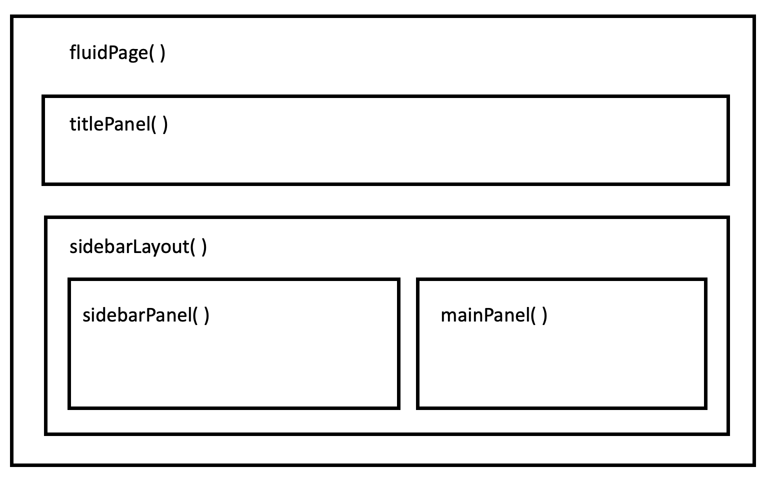
Figure 3. Wireframe diagram displaying the structure of the sidebar layout.
The next step is to fill the ui element with the components necessary to render this sidebar layout. First, use the titlePanel element to give your application a title, and add the sidebar element. Within the fluidPage() object, delete the ‘Hello World’ message and replace with the following:
  titlePanel("Newspaper Map"),

  sidebarLayout()
Following this, populate the layout with specific parts of the webpage, components called sidebarPanel() and mainPanel(). Do this by placing them within sidebarLayout().
The full UI element should now look like this:
ui = fluidPage(

  titlePanel("Newspaper Map"),

  sidebarLayout(

    sidebarPanel = sidebarPanel(),
    mainPanel = mainPanel()

  )
)
You’ll notice that these nested commands correspond to the layout of the wireframe diagram in Figure 3 above.
Add a ‘Widget’: the sliderInput Control
In Shiny, users update values using various interactive, customisable controls known as ‘widgets’. The full list can be found in the Shiny widget gallery. The widget you’re going to use is called sliderInput(). This will display an interactive sliding bar with a large number of options, such as the minimum, maximum and starting value(s). You can also set the step and format of the numbers (type ?sliderInput in the console to get a full list of options and explanations). Here you’ll make one with a minimum year of 1620 (the earliest data point in the title list), and a maximum of 2019 (the most recent).
The starting (default) value can be a single number, or a vector of two numbers. If the latter is used, the slider will be double-sided, with a first and second value. This is what we want to use, so that a user can specify a range of years.
The following code will create a slider with two draggable ends, set by default to 1700 and 1750:
sliderInput('years', 'Years', min = 1621, max = 2000, value = c(1700, 1750))
Insert this code between the parentheses of the sidebarPanel = sidebarPanel( ) command in your script. If you get lost or need to debug, take a look at the finished code provided at the end of this lesson.
At this point, run the application to see how the slider looks. You should see a grey panel on the left (the sidebar panel), containing the slider widget. If you hover over the slider, you’ll notice that you can drag each end (to select a range size) and you can also drag the middle (which will move the entire slider over a window of the selected range size).
Figure 4. Animated gif demonstrating the functionality of the slider input widget.
Put the leafletOutput in the mainPanel Element
In Shiny, you need to let the UI know it should display an output (some kind of R element, such as a table of data or a plot, or something as simple as a line of text) created in the server code. This is done by creating an element in the UI from the *Output family of commands. Each R element you can display in Shiny has its own *Output command: here, you’ll use leafletOutput(), which tells the UI to create a Leaflet map. leafletOutput has one required argument: its output ID. This label will be used to match the UI element to the actual map object you’ll create in the server code later. Set this label as ‘map’. Insert the following code between the parentheses of mainPanel():
leafletOutput(outputId = 'map')
Creating the Server Logic
Next you need to write the logic to create an object which will be displayed in the UI. This has two parts. First, you’ll create a reactive element, which, as explained above, is a special object which will listen for changes to the user input, and remake itself as necessary. Second, you’ll create an output which will contain the interactive map itself.
Create the reactive for the Leaflet map
First, create the reactive element. In this case, it will be a special type of geographic dataset called a simple features object. This format has been covered in a previous Programming Historian lesson, ‘Using Geospatial Data to Inform Historical Research in R’.
Whenever the user changes the variables in the date slider in any way, your app will run through a set of commands:
-
Filter the title list to the set of dates selected by the user
-
Make a count of the number of times each place occurs in this filtered list
-
Match the places to a set of coordinates using a join
-
Convert the result into a simple features object
To create a reactive object called map_df, add the following code within the curly braces of the server component:
map_df = reactive({

  title_list %>%
    filter(first_date_held > input$years[1] & first_date_held < input$years[2]) %>%
    count(coverage_city, name = 'titles') %>%
    left_join(coordinates_list, by = 'coverage_city')%>%
    filter(!is.na(lng) & !is.na(lat)) %>%
    st_as_sf(coords = c('lng', 'lat')) %>%
    st_set_crs(4326)

})
This code performs the following functions:
1. Filter the newspapers dataset using the command filter(), using the values from the sliderInput widget. These values are accessed using input$<LABELNAME>, which in this case is input$years, though there is a further complication to note. Remember you set the value of the sliderInput to a vector of length two, so that a range could be selected? The two numbers of this range are stored in input$years[1] and input$years[2]. These are the values which you need to access in order to filter the data. The filter function returns rows of a dataframe where a specified set of conditions are true: in this case, where the column first_date_held is greater than the first value, and lesser than the second.
2. count() on this filtered dataset to produce a dataframe of each city and a tally of the times they occur. Specify the name of the new column containing the tallies with the argument name =.
3. Perform a join (a type of merge which matches two dataframes together based on a common key) to merge the coordinates dataframe to the counts dataframe using left_join(). You should specify the key on which to join, which is coverage_city.
4. There are a small number of newspaper titles without lat/long coordinates, which would cause an error when creating the geographic object. Filter these out with filter(!is.na(lat) & !is.na(lng))
5. Finally, turn it into a simple features object, using st_as_sf(). To do this, specify the lat/long coordinates columns it should use using coords, and then use st_set_crs to set a coordinate reference system.4
This simple features dataframe can be accessed in any reactive context by Shiny using map_df() and can be used by multiple outputs at once: for example you could build an app which displays both a map and a bar chart, each using the same reactive object.
Create the Leaflet Map
The last thing to do is to create the map itself. This is done using the library leaflet, which allows for interactive, zoomable maps. It works particularly well with Shiny. Add the following code within the server() element, just underneath the map_df reactive element:
output$map = renderLeaflet({

  leaflet() %>%
    addTiles() %>%
    setView(lng = -5, lat = 54, zoom = 5)

})
There are some quite complex things going on here so it is important to go through the code in detail. In Shiny, you create reactivity by connecting inputs to outputs.
Inputs, in this context, are the variables adjusted by the user. Remember the sliderInput() you created in the UI above, with the label ‘years’? We’ve already seen that the value for it is stored by Shiny in the variable input$years.
Outputs are the R expressions which tell Shiny what to display in the UI and are created, in the server, with the variable name output$*. Outputs need to be matched to a UI *Output element. In the UI, you created a leaflet output with the label map using the code leafletOutput('map'). This should be matched to an output in the server named output$map.
In turn, this output$map variable should be set to a Shiny render* function, which tells Shiny what kind of object is to be rendered in the UI. The one we need is called renderLeaflet, which tells the UI to output a map created by the leaflet library. The renderLeaflet object has both parentheses and curly braces, just like the reactive object we created above.
The Leaflet map itself will be created within this. First, add the function leaflet(). Next, add the default tiles (the zoomable map images) using addTiles(). Next, set the default map position and zoom to Britain and Ireland using the command setView(lng = -5, lat = 54, zoom = 5).
Draw Points using the Reactive Dataframe
Pause here and run the application again. All being well, you should see an interactive map of Britain and Ireland to the right of the slider. You can zoom and scroll it, though not much else. It needs to be populated with points representing the count of titles from each place.
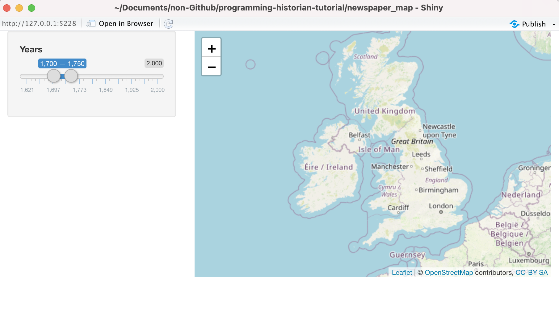
Figure 5. Screenshot of the application with Leaflet map and slider input widget.
To do this, use the command addCircleMarkers(), which adds a graphical layer of circles to the leaflet map, with coordinates taken from a geographic data object. Using the %>% pipe, add the following after the addCircleMarkers() function (see the final code if you’re not sure where this should go):
%>%
  addCircleMarkers(data = map_df(), radius = ~sqrt(titles))
Here is the crucial bit: instead of a fixed data source, the above specifies that addCircleMarkers should use the reactive dataframe we created earlier, with the argument data = map_df(). Notice that unlike regular variables in R, this has a pair of parentheses after it, denoting that it is a special reactive variable. Each time the application notices a change to this reactive object, it will redraw the map with the new data.
At this point you can also set the radius of the circles to correspond to the column containing the count of titles for each place, using radius = ~sqrt(titles). We use the square root, because that makes the area of the circles correctly proportional to the count.
Test the Application
It’s time to run the application again. Now, there should be variously-sized circles dotted across the map. Try moving or dragging the sliders - the map should update with every change. Congratulations, you’ve made your first Shiny app!
Figure 6. Animated gif demonstrating the Leaflet map updating as the values in the slider input widget are changed.
Improving the Application
To learn more about Shiny and Leaflet, you could try adding some of the following features to your application:
First, add an additional user input to filter the map data. Using another widget, selectInput, you could allow a user to display data from just one of the four countries in the title list. Type ?selectInput into the console to get help on the parameters you need to do this correctly. Additional inputs can be placed under the existing sliderInput, separated by a comma.
Next, add some elements to the Leaflet map. A full list of options can be found using ?circleMarkers in RStudio. For example, you can add a label to the points with label = coverage_city.
You’ll notice that every time you move the slider, the entire map redraws and resets its view, which isn’t very elegant. This can be fixed using another function called leafletProxy. In essence, create an empty Leaflet map (without the circleMarkers) as above. Then in another reactive context, observe, you’ll add the code to redraw the changing parts of the map, using leafletProxy. The instructions for how to do this can be found on Leaflet’s docs.
Conclusion
Interactive visualisations can help to bring new insights to historical data. In this tutorial we made use of some powerful R packages, such as the tidyverse and leaflet, and were able to use these in an interactive environment, rather than having to prepare all the data in advance. We learned how and why we might use reactive programming, which allows us to create dynamic R code where user inputs take the place of fixed variables.
This approach can be easily adapted to suit a range of different data formats and modes of analysis. The relatively low barrier to entry makes it easy to create quick applications which can make working with large-scale data less painful. Shiny applications are also a useful way to share some of the benefits of the programming capabilities of R with a non-technical audience or project team members. It’s relatively easy to create an application that will allow a user to visualize their own data analysis with R, without having to actually code or use the command line.
Final code
library(tidyverse)
library(shiny)
library(sf)
library(leaflet)

title_list = read_csv('BritishAndIrishNewspapersTitleList_20191118.csv')

coordinates_list = read_csv('newspaper_coordinates.csv')

ui = fluidPage(

  titlePanel("Newspaper Map"),

  sidebarLayout(

    sidebarPanel = sidebarPanel(sliderInput('years', 'Years', min = 1621, max = 2000, value = c(1700, 1750))),
    mainPanel = mainPanel(

      leafletOutput(outputId = 'map')

    )
  )

)

server = function(input, output){

  map_df = reactive({

    title_list %>%
      filter(first_date_held > input$years[1] & first_date_held < input$years[2]) %>%
      count(coverage_city, name = 'titles') %>%
      left_join(coordinates_list, by = 'coverage_city')%>%
      filter(!is.na(lng) & !is.na(lat)) %>%
      st_as_sf(coords = c('lng', 'lat')) %>%
      st_set_crs(4326)

  })

  output$map = renderLeaflet({

    leaflet() %>%
      addTiles() %>%
      setView(lng = -5, lat = 54, zoom = 5) %>%
      addCircleMarkers(data = map_df(), radius = ~sqrt(titles))

  })


}

shinyApp(ui, server)
End Notes
-
Yann Ryan and Luke McKernan, “Converting the British Library’s Catalogue of British and Irish Newspapers into a Public Domain Dataset: Processes and Applications,” Journal of Open Humanities Data 7, no. 0 (January 22, 2021): 1, https://doi.org/10.5334/johd.23. ↩
-
Legal Deposit was a mechanism by which publishers were obliged to give the British Museum (and subsequently the British Library) a copy of any book produced, including newspapers. ↩
-
The server object is actually an R list with all the inputs stored in the first element, called input, and all the outputs stored in the second element, called output. ↩
-
Because there are various ways to transform a globe into a 2D representation, displaying geographic data correctly requires setting a coordinate reference system. 4326 is a commonly-used one for worldwide geographic data. ↩