
Contents
- Introduction
- A Quick Introduction to Machine Learning
- An In-Depth Guide to Computer Vision using Deep Learning
- Part One Conclusion
- Appendix: A Non-Scientific Experiment Assessing Transfer Learning
- Endnotes
Introduction
While most historians would agree that (modern) representation is shaped by multimodal media —i.e., media, such as the newspaper, television or internet, that combine several modes— the fields of digital humanities and digital history remain dominated by textual media and the wide variety of methods available for its analysis1. Modern historians have frequently been accused of neglecting non-textual forms of representation, and digital humanists in particular have dedicated themselves to exploring textual sources. Many have used Optical Character Recognition (OCR); a technology which renders digitised text machine-readable, alongside techniques stemming from the field of Natural Language Processing (NLP), to analyse the contents and context of language within large documents. The combination of these two has shaped the central methodological innovation of the field of digital history: the ability to ‘distant read’ large corpora and discover large-scale patterns.2
Over the last ten years, the field of computer vision, which seeks to gain a high-level understanding of images using computational techniques, has seen rapid innovation. For example, computer vision models can locate and identify people, animals and thousands of objects included in images with high accuracy. This technological advancement promises to do the same for image recognition that the combination of OCR/NLP techniques has done for texts. Put simply, computer vision opens up a part of the digital archive for large-scale analysis that has remained mostly unexplored: the millions of images in digitised books, newspapers, periodicals, and historical documents. Consequently, historians will now be able to explore the ‘visual side of the digital turn in historical research’.3
This two-part lesson provides examples of how computer vision techniques can be applied to analyse large historical visual corpora in new ways and how to train custom computer vision models. As well as identifying the contents of images and classifying them according to category —two tasks which focus on visual features— computer vision techniques can also be used to chart the stylistic (dis)similarities between images.
It should be noted, however, that computer vision techniques present historians with a set of theoretical and methodological challenges. First, any application of computer vision techniques to historical corpora should start from a carefully formulated historical question and, as a result, include a discussion of scale. In short: why is it important that we answer the question and why are computer vision techniques necessary to answer it?
Second, following discussions in the field of machine learning fairness4,5, which seek to address the question of bias in machine learning (ML), historians should be conscious of the fact that computer vision techniques shed light on certain parts of visual corpora, but might overlook, misidentify, misclassify, or even obscure, other parts. As historians, we have long been aware that we look at the past from our own time, and therefore any application of computer vision techniques should include a discussion of possible ‘historical bias’. Because (most) computer vision models are trained on contemporary data, we run the risk of projecting the time-specific biases of this data onto the historical record. Whilst it is beyond the scope of this two-part lesson to explore the question of bias fully, it is something that should be kept in mind.
Lesson Aims
This two-part lesson aims to:
- Provide an introduction to deep learning-based computer vision methods for humanities research. Deep learning is a branch of machine learning (something we’ll discuss in more detail in the lessons)
- Give an overview of the steps involved in training a deep learning model
- Discuss some of the specific considerations around using deep learning/computer vision for humanities research
- Help you decide whether deep learning might be a useful tool for you
This two-part lesson does not aim to:
- Reproduce other more generic introductions to deep learning, though it does cover some of the same material
- Cover every detail of deep learning and computer vision; computer vision and deep learning are vast topics, and it isn’t possible to cover everything here
Suggested Prior Skills
- Familiarity with Python or another programming language will be important for following these lessons. Specifically, it would be beneficial to understand how to use variables, indexing, and have some familiarity with using methods from external libraries.
- We assume familiarity with Jupyter Notebooks i.e., knowing how to run code included in the notebook. If you are unfamiliar with notebooks, you may find the Introduction to Jupyter Notebooks Programming Historian lesson a helpful resource in conjunction with these lessons.
- There is some use of external Python libraries in this tutorial, but previous knowledge isn’t necessary because the steps involved in using these libraries will be explained as they are used.
Lesson Setup
We suggest approaching this two-part lesson in two stages:
- First, read through the materials on this page, to gain familiarity with the key conceptual issues and the overall workflow for training a computer vision model
- Second, we recommend that you run the code for this lesson through the accompanying Jupyter Notebook on Google Colab, which works well for the exploratory approch we will be following.
In this two-part lesson we will be using a deep learning based approach to computer vision. The process of setting up an environment for doing deep learning has become easier but can still be complex. We have tried to keep this setup process as simple as possible, and recommend a fairly quick route to start running the lesson’s code.
Running the Notebook
You can run the lesson code in a variety of different ways, but we strongly encourage you to use the ‘cloud’ set-up instructions as opposed to setting things up locally. This is for a several reasons:
- The set-up process for using deep learning in a cloud environment can be much simpler than trying to set things up locally. Many laptops and personal computers won’t have this type of hardware available and the process of installing the necessary software drivers can be time consuming.
- The code in this lesson will run much more quickly when a specific type of Graphical Processing Unit (GPU) is available. This will allow for an interactive approach to working with models and outputs.
- GPUs are more energy efficient for some tasks compared to Central Processing Units (CPUs), including the type of tasks we will work with in these lessons.
Google Colab
Google Colab is a free cloud service that supports Jupyter notebooks and provides free access to computing resources including GPUs.
To run the lesson code on Google Colab you will need to:
- Create a free account on Google if you don’t already have one, or log in to your existing account. A Google account is required to save and run notebooks on Colab.
- Open the notebook and click the Open in Colab button.
- Once the notebook is opened, you may want to save a copy to your own Google Drive. You can do this by selecting File > Save a copy in Drive.
-
To use a GPU, go to Runtime > Change runtime type, then under the
Hardware acceleratordropdown, select a GPU option (e.g. T4 GPU) and click Save. This will enable GPU acceleration for your notebook. Colab occasionally changes which type of GPUs they make available.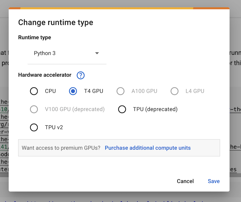
Figure 1. The Google Colab ‘Runtime’ settings menu
- The interface for Colab notebooks should be familiar if you have used Jupyter notebooks before. To run a cell containing code, click the play button on the left side of the cell or, if the cell is selected, use Shift + Enter.
- Remember to disconnect your runtime once you have finished working with the notebooks to avoid using up your allocation of time. You can do this by selecting Runtime > Manage Sessions and then selecting Terminate for your active session.
Google Colab has further documentation on using their notebooks as well as a useful FAQ section for common questions and efficient usage tips.
Local Setup
If you don’t want to use one of the cloud setup instructions you can follow instructions for setting up this lesson locally.
A Quick Introduction to Machine Learning
Before moving to the first practical example, it might be useful to briefly review what is meant by ‘machine learning’. Machine learning aims to allow computers to ‘learn’ from data instead of being explicitly programmed to do something. For example, if we want to filter out spam emails there are a few different approaches we can take. One approach could be to read through examples of ‘spam’ and ‘non-spam’ emails to see if we can identify signals indicating that an email is spam. We might, for example, come up with keywords which we think will be likely to indicate spam. Then we could write a program that does something like this for each email received:
count number spam_words in email:
    if number spam_words >= 10:
        email = spam
In contrast, a machine learning approach would train a machine learning algorithm on labeled examples of emails which are ‘spam’ or ‘not spam’. This algorithm would, over repeated exposure to examples, ‘learn’ patterns which indicate the email type. This is an example of ‘supervised learning’, a process in which an algorithm is exposed to labeled data, and is what this tutorial will focus on. There are different approaches to the managing this training process, some of which we will cover in this two-part lesson. Another type of machine learning which doesn’t require labelled examples is ‘unsupervised learning’.
There are advantages and disadvantages to machine learning. Some advantages in our email example include not having to manually identify what indicates if an email is spam or not. This is particularly useful when signals might be subtle or hard to detect. If the characteristics of spam emails were to change in the future, you wouldn’t need to rewrite your entire program but could instead re-train your model with new examples. Some disadvantages include the requirement for labeled examples which can be time consuming to create. One major limitation of machine learning algorithms is that it can be difficult to understand how they made a decision i.e., why an email was labeled spam or not. The implications of this vary depending on how much ‘power’ the algorithm is given in a system. For example, the potential negative impact from an algorithm making automated decisions about a loan application are likely to be much higher than an algorithm making unhelpful recommendation for a film from a streaming service.
Training an Image Classification Model
Now that we have a general understanding of machine learning, we’ll move to our first example of using deep learning for computer vision. In this example, we will build an image classifier that assigns images to one of two categories based on labeled training data.
The Data: Classifying Images from Historical Newspapers
In this two-part lesson, we will work with a dataset derived from the “Newspaper Navigator”. This dataset consists of extracted visual content for 16,358,041 digitised historic newspaper pages drawn from the Library of Congress’ Chronicling America collection.
A computer vision model assigned these images one of seven categories, including photographs and advertisements.
The Newspaper Navigator data was created using an object detection deep learning model. This model was trained on annotations of first world war-era Chronicling America pages, including annotations made by volunteers as part of the Beyond Words crowdsourcing project.6
If you want to find out more about how this dataset was created you may want to read the journal article describing this work, or look at the GitHub repository which contains the code and training data. We won’t be replicating this model. Instead, we will use the output of this model as the starting point for creating the data we use in this tutorial. Since the data from Newspaper Navigator is predicted by a machine learning model it will contain errors; for now, we will accept that the data we are working with is imperfect. A degree of imperfection and error is often the price we have to pay if we want to work with collections ‘at scale’ using computational methods.
Classifying Newspaper Advertisements
For our first application of deep learning, we’ll focus on classifying images predicted as adverts (remember this data is based on predictions and will contain some errors). More specifically, we’ll work with a sample of images in adverts covering the years 1880-5.
Detecting if Advertisements Contain Illustrations
If you look through the advert images, you will see that some of the adverts contain only text, whilst others have some kind of illustration.
An advert with an illustration7:
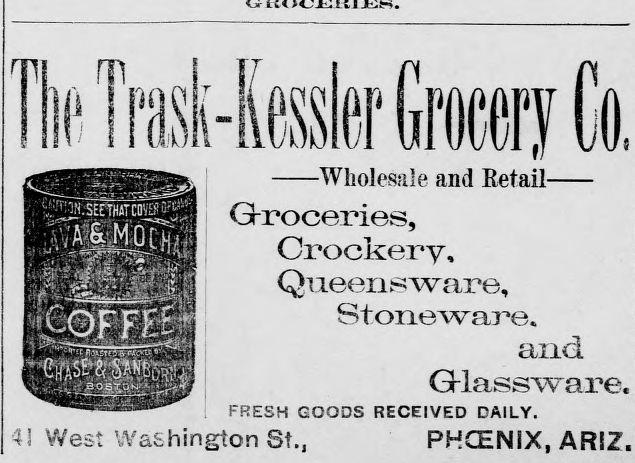
Figure 2. An example of an illustrated advert
An advert without an illustration8:

Figure 3. An example of a text only advert
Our classifier will be trained to predict which category an advert image belongs. We might use this to help automate finding adverts with images for further ‘manual’ analysis. Alternatively, we may use this classifier more directly to quantify how many adverts contained illustrations in a given year and discover whether this number changed over time, along with how it was influenced by other factors such as the place of publication. The intended use of your model will impact the labels you choose to train it on and how you choose to assess whether a model is performing sufficiently well. We’ll dig into these issues further as we move through this two-part lesson.
An Introduction to the fastai Library
fastai is a Python library for deep learning “which provides practitioners with high-level components that can quickly and easily provide state-of-the-art results in standard deep learning domains, and provides researchers with low-level components that can be mixed and matched to build new approaches”9. The library is developed by fast.ai (notice the dot!), a research organisation that aims to make deep learning more accessible. Alongside the fastai library, fast.ai also organises free courses and carries out research.
There are a few reasons why fastai was chosen for this tutorial:
- It is focused on making deep learning accessible, particularly through the design of library’s API.
- It facilitates the use of techniques that don’t require a large amount of data or computational resources.
- Many best practices are implemented as ‘defaults’, helping achieve good results.
- There are different levels at which you can interact with the library depending on how much you need to change lower-level details.
- The library sits on top of PyTorch which makes it relatively simple to use existing code.
Although this tutorial focuses on fastai, many of the techniques shown are applicable across other frameworks too.
Creating an Image Classifier in fastai
The next section will outline the steps involved in creating and training a classification model to predict whether an advert is text-only or also contains an illustration. Briefly, the steps will be:
- Load the data
- Create a model
- Train the model
These steps will be covered fairly quickly; don’t worry if you feel you are not following everything in this section, the lesson will get back to what is happening in more detail when we get to the the workflow of a computer vision problem section.
The first thing we’ll do is import the required modules from the fastai library. In this case, we import vision.all since we are working on a computer vision task.10
from fastai.vision.all import *
We will also import Matplotlib, a library for creating visualisations in Python. We will ask Matplotlib to use a different style using the style.use method.
%matplotlib inline
import matplotlib.pyplot as plt
plt.style.use('seaborn-v0_8')
Loading the Data
There are a number of ways in which data can be loaded using the fastai library. The advert data consists of a folder which contains the image files, and a CSV file which contains a column with paths to the images, and the associated label:
| file | label |
|---|---|
| kyu_joplin_ver01_data_sn84037890_00175045338_1900060601_0108_007_6_97.jpg | text-only |
There are various ways in which we could load this type of data using fastai. In this example we’ll use ImageDataLoaders.from_csv. As the name suggests the from_csv method of ImagDataLoaders loads data from a CSV file. We need to tell fastai a few things about how to load the data to use this method:
- The path to the folder where images and CSV file are stored
- The coloumns in the CSV file which contain the labels
- One ‘item transform’
Resize()to resize all the images to a standard size
We’ll create a variable ad_data which will be used to store the paramaters for how to load this data:
ad_data = ImageDataLoaders.from_csv(
    path="ads_data/",  # root path to csv file and image directory
    csv_fname="ads_upsampled.csv/",  # the name of our csv file
    folder="images/",  # the folder where our images are stored
    fn_col="file",  # the file column in our csv
    label_col="label",  # the label column in our csv
    item_tfms=Resize(224, ResizeMethod.Squish),  # resize imagesby squishing so they are 224x224 pixels
    seed=42,  # set a fixed seed to make results more reproducible
)
It is important to make sure that data has been loaded correctly. One way to check this quickly is to use show_batch() method on our data. This will display the images and the associated labels for a sample of our data. The examples you get back will be slightly different to those here.
ad_data.show_batch()
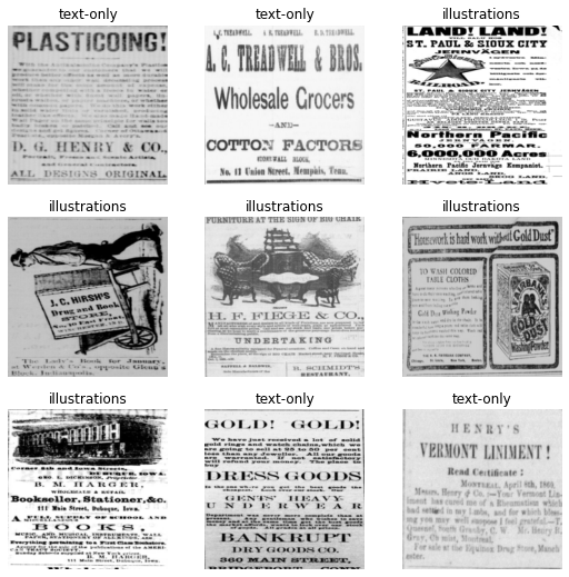
Figure 4. The output of ‘show_batch’
This is a useful way of checking that your labels and data have been loaded correctly. You can see here that the labels (text-only and illustration) have been associated correctly with how we want to classify these images.
Creating the Model
Now that fastai knows how to load the data, the next step is to create a model with it. To create a model suitable for computer vision we will use the vision_learner function. This function will create a ‘Convolutional Neural Network’, a type of deep learning model often used for computer vision applications. To use this function you need to pass (at a minimum):
- The data the model will use as training data
- The type of model you want to use
This is already sufficient for creating a computer vision model in fastai, but you may also want to pass some metrics to track during training. This allows you to get a better sense of how well your model is performing the task you are training it on. In this example, we’ll use accuracy as the metric.
Let’s create this model and assign it to a new variable learn:
learn = vision_learner(
    ad_data,  # the data the model will be trained on
    resnet18,  # the type of model we want to use
    metrics=accuracy,  # the metrics to track
)
Training the Model
Although we have created a vision_learner model, we haven’t actually trained the model yet. This is done using the fit method. Training is the process which allows the computer vision model to ‘learn’ how to predict the correct labels for the data. There are different ways we can train (fit) this model. To start with, we’ll use the fine_tune method. In this example the only thing we’ll pass to the fine tune method is the number of epochs to train for. Each pass through the entire dataset is an ‘epoch’. The amount of time the model takes to train will depend on where you are running this code and the resources available. Again, we will cover the details of all of these components below.
learn.fine_tune(5)
| epoch | train_loss | valid_loss | accuracy | time |
|---|---|---|---|---|
| 0 | 0.971876 | 0.344096 | 0.860000 | 00:06 |
| epoch | train_loss | valid_loss | accuracy | time |
|---|---|---|---|---|
| 0 | 0.429913 | 0.394812 | 0.840000 | 00:05 |
| 1 | 0.271772 | 0.436350 | 0.853333 | 00:05 |
| 2 | 0.170500 | 0.261906 | 0.913333 | 00:05 |
| 3 | 0.125547 | 0.093313 | 0.946667 | 00:05 |
| 4 | 0.107586 | 0.044885 | 0.980000 | 00:05 |
When you run this method you will see a progress bar showing how long the model has been training and the estimated time remaining. You will also see a table which displays some other information about the model, such as our tracked accuracy metric. You can see that in this example we got an accuracy greater than 90%. When you run the code yourself, the score you get may be be slightly different.
Results
While deep learning techniques are commonly perceived as needing large amounts of data and extensive computing power, our example shows that for many applications smaller datasets suffice. In this example, we could have potentially used other approaches; the aim here was not to show the best solution with this particular dataset but to give a sense of what is possible with a limited number of labeled examples.
An In-Depth Guide to Computer Vision using Deep Learning
Now that we have an overview of the process we’ll go into more detail about how this process works.
The Workflow of a Supervised Computer Vision Problem
This section will start to dig into some of the steps involved in the process of creating a deep learning based computer vision model. This process involves a range of steps, only some of which are directly about training models. A high-level illustration of a supervised machine learning pipeline might look like this:
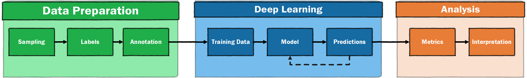
Figure 5. A high level illustration of a supervised machine learning pipeline
We can see that there are quite a few steps before and after the model training phase of the workflow. Before we get to training a model, we need data. In this lesson, image data has already been prepared so you didn’t need to worry about this step. However, when you move to using computer vision for your own research questions, it is unlikely that there will an existing dataset for your exact use case. As a result, you will need to create this data yourself. The process of getting access to data will vary depending on the type of images you are interested in working with and where they are held. Some heritage collections are making bulk collections of images data available, whilst others largely make images available only via a ‘viewer’. The increasing adoption of the IIIF standard is also making the process of working with images held by different institutions simpler.
Once you have a collection of images to work with, the next step (if using supervised learning) will be to create some labels for this data and train the model. This process will be discussed in more detail below. Once a model has been trained you will get out some predictions. These predictions are ‘scored’ using a range of potential metrics, some of which we’ll explore further in Part 2 of this lesson.
Once a model has reached a satisfactory score, its outputs may be used for a range of ‘interpretative” activities. Once we have predictions from a deep learning model there are different options for what to do with these. Our predictions could directly inform automated decisions (for example, where images are to be displayed within a web collection), but it is more likely that those predictions will be read by a human for further analysis. This will particularly be the case if the intended use is to explore historical phenomena.
Training a Model
Zooming in on the deep learning part of the workflow, what does the training process look like?
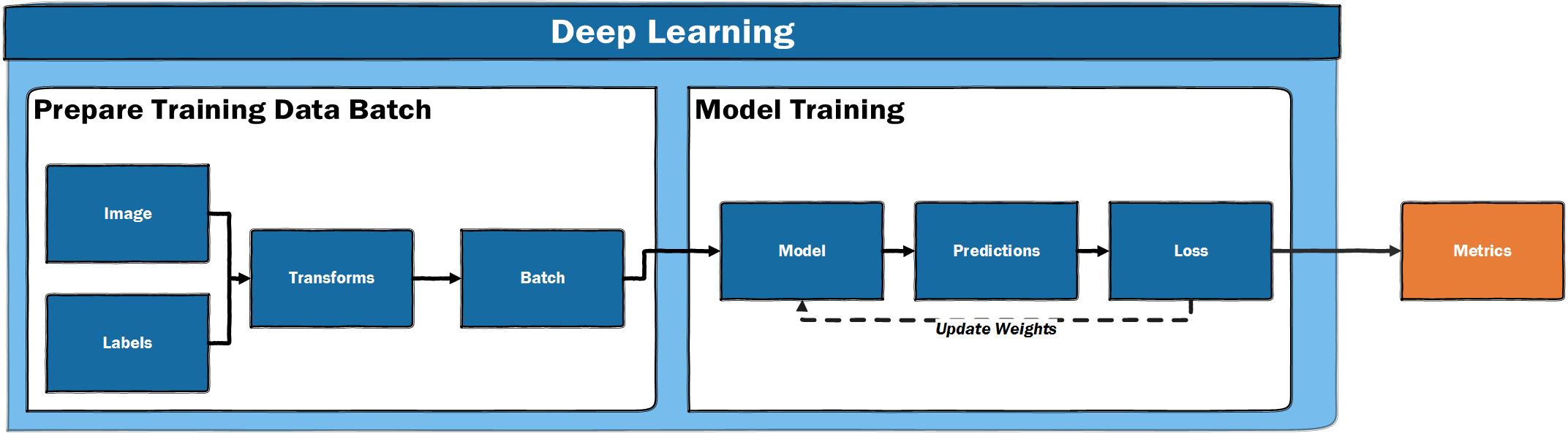
Figure 6. The deep learning training loop
A high-level summary of the training loop for supervised learning: start with some images and labels, do some preparation to make the input suitable for a deep learning model, pass the data through the model, make predictions for the labels, calculate how wrong the predictions are, update the model with the aim of generating better predictions next time. This process is repeated a number of times. During this training loop, metrics are reported which let the human training the model evaluate how well the model is doing.
This is obviously a high-level summary. Let’s look at each step in the training loop one at a time. Although the next section will show these steps using code, don’t worry too much if it doesn’t all sink in at first.
Input Data
Starting with the inputs, we have images and labels. Although deep learning takes some inspiration from how human cognition works, the way a computer ‘sees’ is very different from a human. All deep learning models take numbers as inputs. Since images are stored on a computer as a matrix of pixel values, this process is relatively simple for computer vision models. Alongside these images, we have a label(s) associated with each image. Again, these are represented as numbers inside the model.
How Much Data?
It is often believed that you need huge amounts of data to train a useful deep learning model, however, this is not always the case. We assume that if you are trying to use deep learning to solve a problem, you have enough data to justify not using a manual approach. The real problem is the amount of labelled data you have. It is not possible to give a definitive answer to “how much data?”, since the amount of training data required is dependent on a broad range of factors. There are a number of things which can be done to reduce the amount of training data required, some of which we will cover in this lesson.
The best approach will likely be to create some initial training data and see how well your model does on it. This will give you a sense of whether a problem is possible to tackle. Furthermore, the process of annotating your data is valuable in itself. For a simple classification task, it might be possible to begin assessing whether a model is worth developing with a few hundred labelled examples (though you will often need more than this to train a robust model).
Preparing Mini Batches
When we use deep learning, it is usually not possible to pass all of our data into the model in one go. Instead, data is split into batches. When using a GPU, data is loaded into GPU memory one batch at a time. The size of this batch can impact the training process but is more often determined by the computational resources you have available.
The reason we use a GPU for training our model is that it will almost always be quicker to train a model on a GPU compared to a CPU due to its ability to perform many calculations in parallel.
Before we can create a batch and load it onto the GPU, we usually need to make sure the images are all the same size. This allows the GPU to run operations effectively. Once a batch has been prepared, we may want to do some additional transformations on our images to reduce the amount of training data required.
Creating a Model
Once we have prepared data so it can be loaded one batch at a time, we pass it to our model. We already saw one example of a model in our first example resnet18. A deep learning model architecture defines how data and labels are passed through a model. In this two-part lesson, we focus on a specific type of deep learning that uses ‘Convolutional Neural Networks’ (CNN).
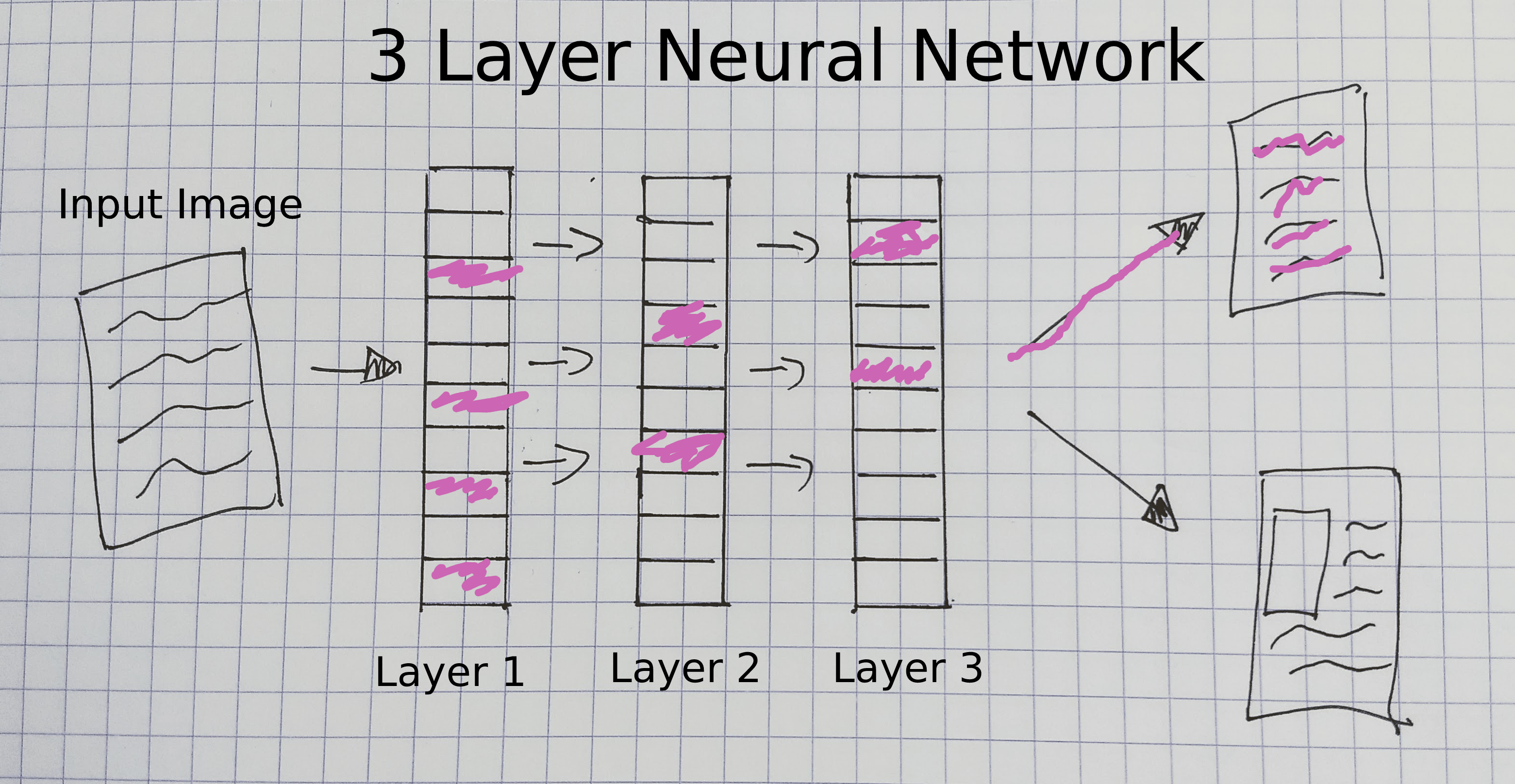
Figure 7. A three layer neural network
This diagram gives a crude overview of the different components of a CNN model. In this type of model, an image is passed through several layers, before predicting an output label for the image (‘text only’ in this diagram). The layers of this model are updated during training so that they “learn” which features of an image predict a particular label. So for example, the CNN we trained on adverts will update the parameters known as “weights” for each layer, which then produces a representation of the image that is useful for predicting whether an advert has an illustration or not.
Tensorflow playground is a useful tool for helping to develop an intuition about how these layers capture different features of input data, and how these features, in turn, can be used to classify the input data in different ways.
The power in CNNs and deep learning comes from the ability of these layers to encode very complicated patterns in data.11 However, it can often be a challenge to update the weights effectively.
Using an Existing Model?
When considering how to create our model we have various options about what to use. One option is to use an existing model which has already been trained on a particular task. You might for example use the YOLO model. This model is trained to predict bounding boxes for a number of different types of objects in an image. Although this could be a valid starting point, there are a number of limitations to this approach when working with historical material, or for humanities questions more broadly. Firstly, the data these models were trained on might be very different from the data you are using. This can impact your model’s performance on your data and result in biases towards images in your data which are similar to the training data. Another issue is that if you use an existing model without any modification, you are restricted to identifying the labels the original model was trained on.
Although it is possible to directly define a CNN model yourself by defining the layers you want your model architecture to include, this is usually not where you would start. It is often best to start with an existing model architecture. The development of new model architectures is an active area of research, with models proving to be well-suited for a range of tasks and data. Often, these models are then implemented by machine learning frameworks. For example, the Hugging Face Transformers library implements many of the most popular model architectures.
Often, we want a balance between starting from scratch and leveraging existing models. In this two-part lesson, we show an approach which uses existing model architectures but modifies the model slightly to allow it to predict new labels. This model is then trained on new data so it becomes better suited to the task we want it to perform. This is a technique known as ‘transfer learning’ which will be explored in the appendix section of this lesson.
Training
Once a model has been created and data prepared, the training process can begin. Let’s look at the steps of a training loop:
-
A model is passed data and labels, one batch at a time. Each time an entire dataset has been passed through a model is known as an ‘epoch’. The number of epochs used to train a model is one of the variables that you will need to control.
-
The model makes predictions for these labels based on the given inputs, using a set of internal weights. In this CNN model, the weights are contained within the layers of the CNN.
-
The model calculates how wrong the predictions are, by comparing the predictions to the actual labels. A ‘loss function’ is used to calculate how ‘wrong’ the model was in its predictions.
-
The model changes internal parameters to try to do better next time. The loss function from the previous step returns a ‘loss value’, often just referred to as the ‘loss’, which is used by the model to update the weights.
A ‘learning rate’ is used to determine how much a model should update based on the calculated loss. This is another one of the important variables that can be manipulated during the training process. In Part 2 of this lesson, we will see one potential way of trying to identify a suitable learning rate for your model.
Validation Data
When we train a deep learning model, we usually do so to make predictions on new unseen data which doesn’t contain labels. For example, we might want to use our advert classifier across all of images for a particular time period to count how many of each type of advert (illustrated or not) appeared in this corpus. We, therefore, don’t want a model that only does well at learning how to classify the training data it is shown. Consequently, we almost always use some form of ‘validation data’. This is data which is used to check that the weights a model is learning on the training data also translate to new data. In the training loop, the validation data is only used to ‘test’ the model’s predictions. The model does not directly use to update weights. This helps ensure we don’t end up ‘overfitting’ our model.
‘Overfitting’ refers to when a model becomes very successful at making predictions on the training data but these predictions don’t generalise beyond the training data. In effect, the model is ‘remembering’ the training data rather than learning more general features to make correct predictions on new data. A validation set prevents this by allowing you to see how well the model is doing on data it hasn’t learned from. Sometimes, an additional split is made of the data which is used to make predictions only at the end of training a model. This is often known as a ‘test’ set. A test set is used to validate model performance for data science competitions, such as those hosted on Kaggle, and to validate the performance of models created by external partners. This helps ensure a model is robust in situations where validation data has deliberately or accidentally been used to ‘game’ the performance of a model.
Transfer Learning
In our first advert classifier, we used the fine_tune() method on our learner for training. What was this doing? You will have seen that the progress bar output two parts. The first epoch was training only the final layers of the model, after this the lower layers of the model were also trained. This is one way in which we can do transfer learning in fastai. The importance of transfer learning has already been discussed in the previous sections. As a reminder, transfer learning uses the ‘weights’ that a model has previously learned on another task on a new task. In the case of image classification, this usually means a model has been trained on a much larger dataset. Often this previous training dataset is ImageNet.
ImageNet is a large database of images which is heavily used in computer vision research. ImageNet currently contains “14,197,122” images with over 20,000 different labels. This dataset is often used as a benchmark for computer vision researchers to compare their approaches. Ethical issues related to the labels and production of ImageNet are explored in The Politics of Images in Machine Learning Training Sets by Crawford and Paglen.4
Why Does Transfer Learning Often Help?
As we have seen, transfer learning works by using a model trained on one task to perform a new task. In our example, we used a model trained on ImageNet to classify images of digitised nineteenth century newspapers. It might seem strange that transfer learning works in this case, since the images we are training our model on are very different from the images in ImageNet. Although ImageNet does have a category for newspapers, these largely consist of images of newspapers in the context of everyday settings, rather than images cropped from the pages of newspapers. So why is using a model trained on ImageNet still useful for a task which has different labels and images to those in ImageNet?
When we looked at the diagram of a CNN model we saw that it is made of different layers. These layers create representations of the input image which pick up on particular features of an image for predicting a label. What are these features? They could be ‘basic’ features, for example simple shapes. Or, they could be more complex visual features, such as facial features. Various techniques have been developed to help visualise the different layers of a neural network. These techniques have found that the earlier layers in a neural network tend to learn more ‘basic’ features, for example they learn to detect basic shapes like circles, or lines, whilst layers further into the network contain filters which encode more complex visual features, such as eyes. Since many of these features capture visual properties useful for many tasks, starting with a model that is already capable of detecting features in images will help detect features which are important for the new task, since these new features are likely to be variants on the features the model already knows rather than new ones.
When a model is created in the fastai library using the vision_learner method, an existing architecture is used as the “body” of the model. The deeper layers added are known as the model’s “head”. The body uses the weights (parameters) learned through training on ImageNet by default. The “head” part takes the output of the body as input before moving to a final layer which is created to fit the training data you pass to vision_learner. The fine_tune method first trains only the head part of the model i.e. the final few layers of the model, before ‘unfreezing’ the lower layers. When these layers are ‘unfrozen’ the weights of the model are updated through the process discussed above under ‘training’. We can also take more active control of how much we train different layers of the model, something we will see as we move through a full pipeline of training a deep learning model.
Suggested Experiments
It is important to develop a sense of what happens when you make changes to the training process. We suggest making a new copy of the lesson notebook and seeing what happens if you make changes. Here are some suggestions:
- Change the size of the input images defined in the
Resizeitem transform in theImageDataLoaders. - Change the model used in
vision_learnerfromresnet18toresnet34. - Change the ‘metrics’ defined in
vision_learner. Some metrics included in fastai can be found in the documentation. - Change the number of ‘epochs’ used in the
fine_tunemethod.
If something ‘breaks’, don’t worry! You can return to the original notebook to get back to a working version of the code. In the next part of the lesson, the components of a deep learning pipeline will be covered in more detail. Investigating what happens when you make changes will be an important part of learning how to train a computer vision model.
Part One Conclusion
In this lesson we:
- Gave a high-level overview of the distinction between rule-based and machine learning-based approaches to tackling a problem.
- Showed a basic example of how to use fastai to create an image classifier with relatively little time and training data.
- Presented an overview of the steps of a deep learning pipeline and identified points in this pipeline where humanities scholars should pay particular attention.
- Ran a crude experiment to try and verify if transfer learning is useful for our computer vision classifier.
In the next part of this lesson, we will build on these points and dive into more detail.
Appendix: A Non-Scientific Experiment Assessing Transfer Learning
The use of deep learning in the context of working with heritage data has not been extensively researched. It is therefore useful to ‘experiment’ and validate whether a particular technique is effective. For example, let’s see if transfer learning will prove to be helpful when training a model to classify nineteenth century newspaper adverts into two categories: those containing images and those without images. To do this, we’ll create a new learner with the same parameters as before but with the pretrained flag set to False. This flag tells fastai not to use transfer learning. We’ll store this in a variable learn_random_start.
learn_random_start = vision_learner(ad_data, resnet18, metrics=accuracy, pretrained=False)
Now that we have created a new learner, we’ll use the same fine_tune method as before and train for the same number of epochs as last time.
learn_random_start.fine_tune(5)
| epoch | train_loss | valid_loss | accuracy | time |
|---|---|---|---|---|
| 0 | 1.303890 | 0.879514 | 0.460000 | 00:04 |
| epoch | train_loss | valid_loss | accuracy | time |
|---|---|---|---|---|
| 0 | 0.845569 | 0.776279 | 0.526667 | 00:05 |
| 1 | 0.608474 | 0.792034 | 0.560000 | 00:05 |
| 2 | 0.418646 | 0.319108 | 0.853333 | 00:05 |
| 3 | 0.317584 | 0.233518 | 0.893333 | 00:05 |
| 4 | 0.250490 | 0.202580 | 0.906667 | 00:05 |
The best acurracy score we achieve when we randomly initialise the weights is ~90%. In comparison, if we go back to our original model, which is stored in a variable learn, and use the validate() method, we get the metrics (in this case accuracy) calculated on the validation set:
learn.validate()
(#2) [0.04488467052578926,0.9800000190734863]
We see that there is a fairly big difference between the two models’ performance. We kept everything the same except the pretrainedflag, which we set to False. This flag determines if the model starts from the weights learned from training on ImageNet or starts from ‘random’ weights.12 This doesn’t conclusively prove that transfer learning works, but it does suggest a sensible default for us to use.
Endnotes
-
Romein, C. Annemieke, Max Kemman, Julie M. Birkholz, James Baker, Michel De Gruijter, Albert Meroño‐Peñuela, Thorsten Ries, Ruben Ros, and Stefania Scagliola. ‘State of the Field: Digital History’. History 105, no. 365 (2020): 291–312. https://doi.org/10.1111/1468-229X.12969. ↩
-
Moretti, Franco. Distant Reading. Illustrated Edition. London ; New York: Verso Books, 2013. ↩
-
Wevers, Melvin, and Thomas Smits. ‘The Visual Digital Turn: Using Neural Networks to Study Historical Images’. Digital Scholarship in the Humanities 35, no. 1 (1 April 2020): 194–207. https://doi.org/10.1093/llc/fqy085. ↩
-
Crawford, K., Paglen, T., 2019. Excavating AI: The Politics of Training Sets for Machine Learning. https://www.excavating.ai (accessed 2.17.20). ↩ ↩2
-
Jo, Eun Seo, and Timnit Gebru. ‘Lessons from Archives: Strategies for Collecting Sociocultural Data in Machine Learning’. In Proceedings of the 2020 Conference on Fairness, Accountability, and Transparency, 306–316. FAT* ’20. New York, NY, USA: Association for Computing Machinery, 2020. https://doi.org/10.1145/3351095.3372829. ↩
-
These annotations include a ‘bounding box’ around images, along with information about the type of image is contained within that bounding box. This object detection model was trained on this data and subsequently used to make predictions across the whole Chronicling America collection. The model extracts images from the page and classifies them into one of seven categories. Lee, Benjamin Charles Germain, Jaime Mears, Eileen Jakeway, Meghan Ferriter, Chris Adams, Nathan Yarasavage, Deborah Thomas, Kate Zwaard, and Daniel S. Weld. ‘The Newspaper Navigator Dataset: Extracting And Analyzing Visual Content from 16 Million Historic Newspaper Pages in Chronicling America’. ArXiv:2005.01583 [Cs], 4 May 2020. https://doi.org/10.48550/arXiv.2005.01583. ↩
-
Arizona republican. [volume] (Phoenix, Ariz.) 1890-1930, March 29, 1895, Page 7, Image 7. Image provided by Arizona State Library, Archives and Public Records; Phoenix, AZ. https://chroniclingamerica.loc.gov/lccn/sn84020558/1895-03-29/ed-1/seq-7/. ↩
-
The Indianapolis journal. [volume] (Indianapolis [Ind.]) 1867-1904, February 06, 1890, Page 8, Image 8. Image provided by Indiana State Library. https://chroniclingamerica.loc.gov/lccn/sn82015679/1890-02-06/ed-1/seq-8/. ↩
-
Howard, Jeremy, and Sylvain Gugger. ‘Fastai: A Layered API for Deep Learning’. Information 11, no. 2 (16 February 2020): 108. https://doi.org/10.3390/info11020108. ↩
-
Using ‘star imports’ is generally discouraged in Python. However, fastai uses
__all__to provide a list of packages that should be imported when using star import. This approach is useful for exploratory work but you may still want to change your imports to be more explicit. ↩ -
Neural Networks are able to theoretically approximate any function. The mathematical proof of this exists in a number of forms under the heading of the “Universal Approximation theorem”. These proofs are not things you will need to know to practically use deep learning. However, if you are interested, a good overview of the idea can be found in a YouTube video. ↩
-
This initialisation isn’t actually random in the fastai framework, and instead uses Kaiming initialization. ↩