
Contents
Overview
Twitter data are widely used for research purposes and are collected through a variety of methods and tools. In this guide, we’ll show you easy methods for acquiring Twitter data, with some gestures toward specific types of spatial and social analyses. More specifically, we will be acquiring unique IDs from Twitter, linking those IDs to detailed data about the tweet texts and the users, and processing that data to make it usable. Then we will be ready to generate insights from the data and analyze them with various methods and tools, such as textual and social network analysis. This process might be attractive to historians, political scientists, public policy experts, sociologists, (and even literary scholars like myself) who want to examine the Twitter discourse and human interaction surrounding historical events, and gain insight into the geographic, chronological, and social elements of twenty-first-century politics.
While this walkthrough proposes a specific workflow that we think is suitable for students and researchers of all experience levels (it was originally conceived as a workshop for first-year undergraduates at Georgia Tech), we will note points in the process where other/more advanced techniques could be substituted. Please note that this guide is aimed at beginners, and thus utilizes several GUIs (Graphical User Interfaces) so as to be more accessible to more people. It is our hope that this will serve as an “on-ramp” to working with Twitter data, thus allowing more researchers insight into the geographical and social dimensions of discourse on Twitter.
TweetSets
First, we need to gather some data. George Washington University’s TweetSets allows you to create your own data queries from existing Twitter datasets they have compiled. The datasets primarily focus on the biggest (mostly American) geopolitical events of the last few years, but the TweetSets website states they are also open to queries regarding the construction of new datasets. We chose TweetSets because it makes narrowing and cleaning your dataset very easy, creating stable, archivable datasets through a relatively simple graphical interface. Additionally, this has the benefit of allowing you to search and analyze the data with your own local tools, rather than having your results shaped by Twitter search algorithms that may prioritize users you follow, etc.
You could, however, substitute any tool that gives you a set of dehydrated tweets. Because tweets can be correlated to so much data, it’s more efficient to distribute dehydrated data sets consisting of unique tweet IDs, and then allow users to “hydrate” the data, linking retweet counts, geolocation info, etc., to unique IDs. More importantly, Twitter’s terms for providing downloaded content to third parties, as well as research ethics, are at play. Other common places to acquire dehydrated datasets include Stanford’s SNAP collections, the DocNow Project and data repositories, or the Twitter Application Programming Interface (API), directly. (If you wonder what an API is, please check this lesson.) This latter option will require some coding, but Justin Littman, one of the creators of TweetSets, does a good job summarizing some of the higher-level ways of interacting with the API in this post.
We find that the graphical, web-based nature of TweetSets, however, makes it ideal for learning this process. That said, if you want to obtain a dehydrated dataset by other means, you can just start at the Hydrating section.
Selecting a Dataset
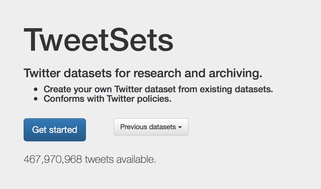
TweetSets start page
If you’re using TweetSets, click “Get Started” and you’ll be able to see a list of all of their existing datasets. Clicking the name of each set will give you more information on it, including its DOI, or Digital Object Identifier, which allows you to reliably locate a digital object (and learn more about how it was created).
When you have decided on the dataset you want to pull from, simply check the checkbox to the left. We’ve chosen a dataset focusing on Hurricane Irma a major storm in the 2017 Atlantic Hurricane Season. As you can see, this will give us just over 17 million tweets as is. If you want to work with multiple datasets, follow the steps for downloading and hydrating each one separately.
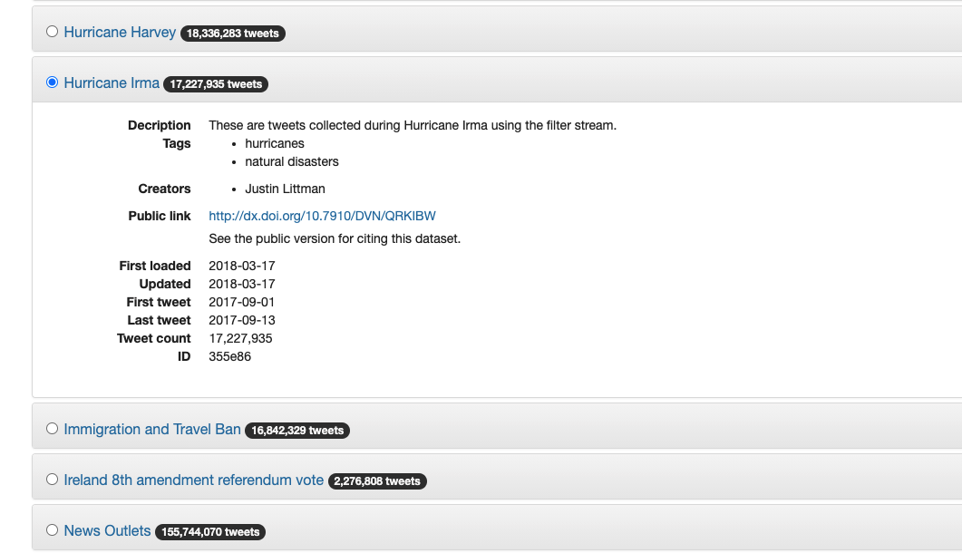
Dataset Selection Page
We’ll filter the dataset to make it easier to work with, but if you’re feeling confident in your data manipulation skills, you can download the whole thing.
Filtering the Dataset with Parameters
On the parameters page, you have the option to limit your dataset by the tweet text content, hashtags used, mentions made, users who posted the tweets, users who are being replied to, the tweet type (original, quote, retweet, or reply), the timeframe during which the tweets were posted, or if they contain things like embedded images or geotags.
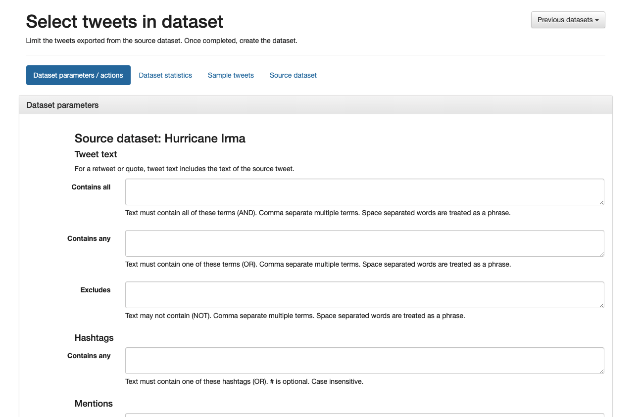
The ‘Parameters’ page
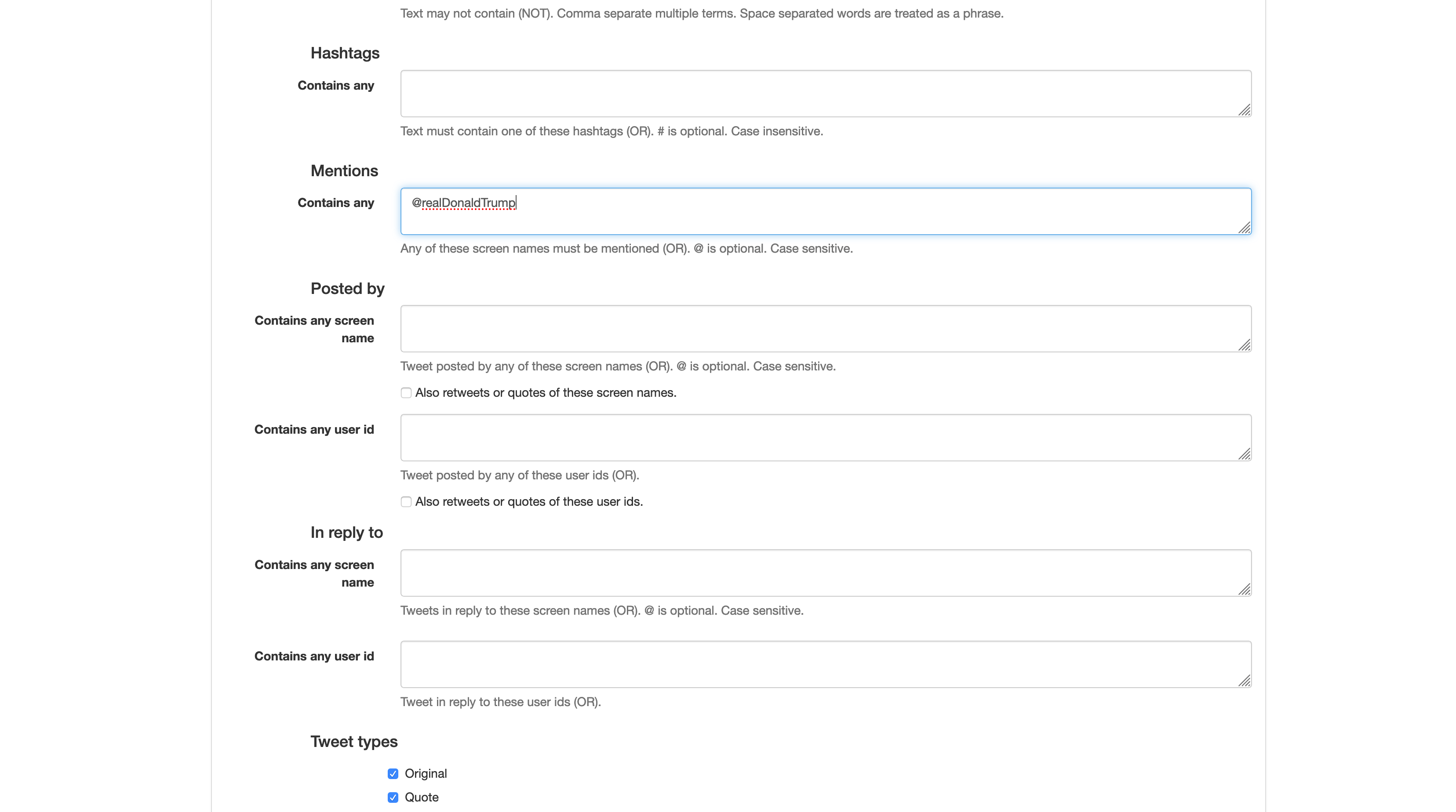
Selecting all tweets that mention @realDonaldTrump.
As you can see above, we’ve chosen to limit our dataset by two parameters. First, we want tweets that mention @realDonaldTrump and second, we want tweets that have geotags or location information. This should give us a good view of who is talking about President Trump in these datasets, and where they are located. You can imagine this kind of data would be good in analyzing how discourse around disasters forms both at ground zero and more broadly.
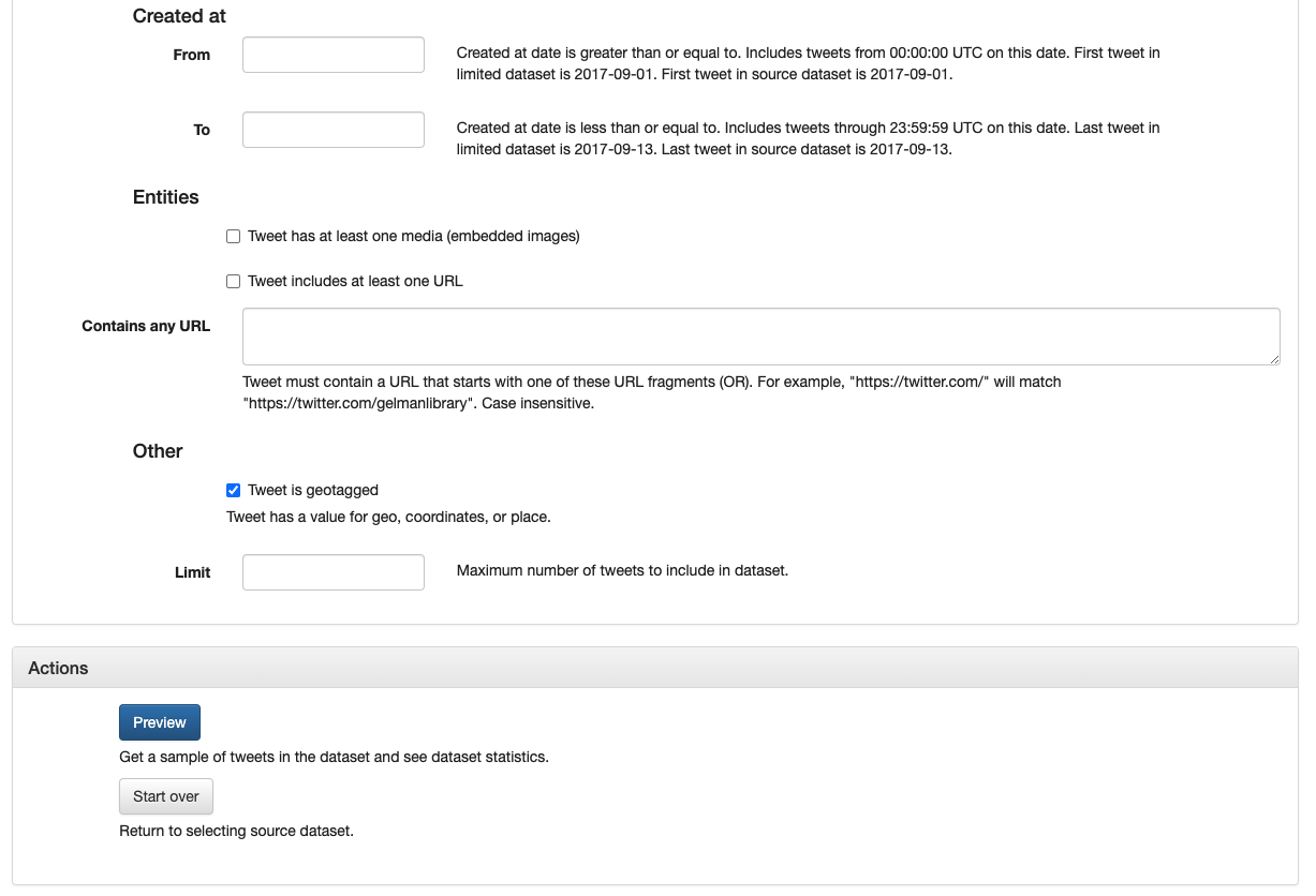
Selecting all geotagged tweets and the Action buttons section
Once you have filled in your desired parameters, select “Preview” to proceed. You will see a sample of the tweets based on your parameters, and, conveniently, the number of tweets your current parameters will return. As you can see, the two parameters we chose have the added benefit of winnowing down the dataset from over seventeen million tweets to just under two thousand: much more manageable. This option is very helpful to make sure you are constructing a dataset that will work for your purposes before you actually go and download a bunch of data. With more advanced tools, you usually have to download and hydrate your data before being able to figure out what is in it.
You can also view some analytics about the dataset, such as the top users (most frequent tweet authors), top mentions, top hashtags, and top URLs. The first 1,000 rows of each of these lists is downloadable from this page.
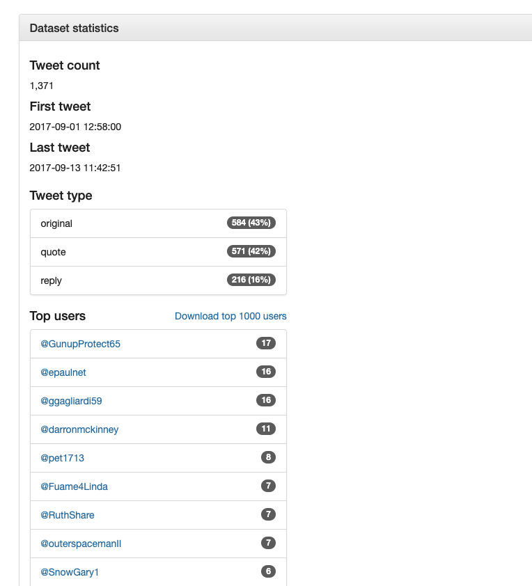
Dataset Preview
The “Create Dataset” option will freeze the parameters and create an exportable dataset. “Start over” will reset your parameters and also return you to the dataset selection page.
Exporting the Dataset
To continue on, press “Create Dataset”, at which point you will need to provide a name. This distinguishes this dataset from others you create on the site, so make it something descriptive.
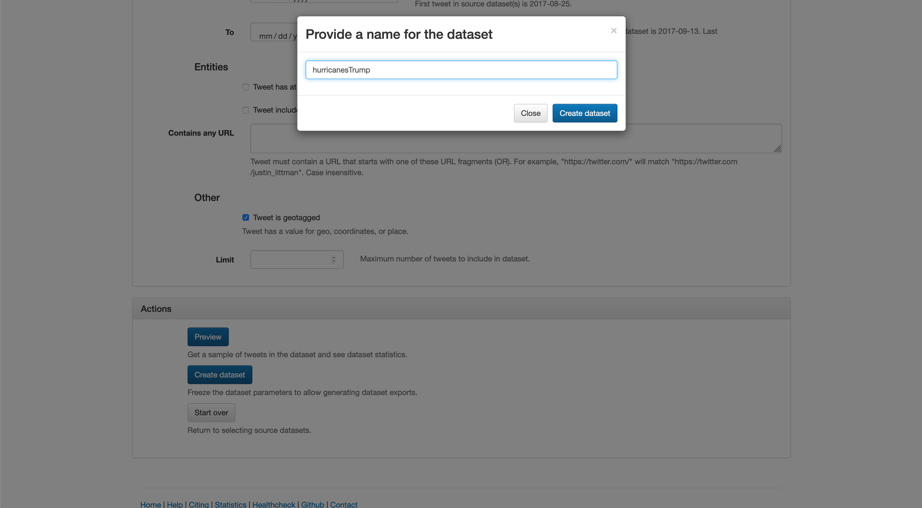
The site prompts you for a name.
Next, select “Generate tweet IDs” and provide an email address so you can be notified when a dataset has been generated. (This can take some time for large datasets.) The file of tweet IDs which will be generated will look similar to other Twitter data files you may encounter from other sources.
Download (and extract) the Tweet ID and Mentions files. Note the instructions for extracting .gz files.
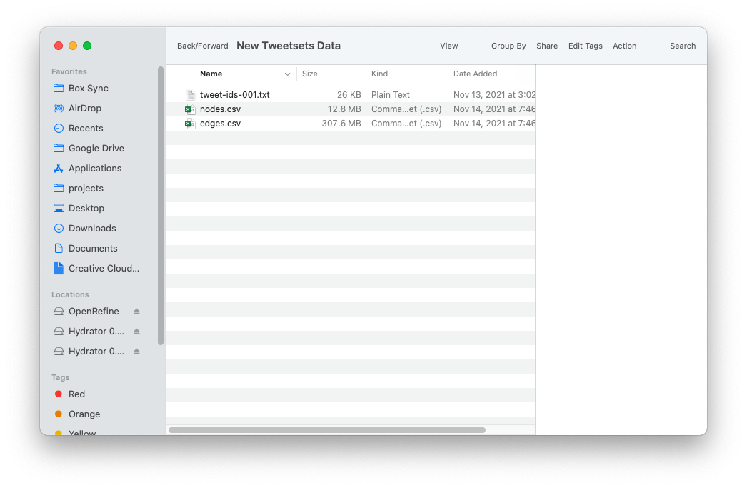
After extraction, your file should look something like this. You might rename the files to indicate the nodes and edges files.
Hydrating
Now that you have a set of tweet IDs, you can hydrate the file using the DocNow Hydrator, a free, open-source piece of hydration software found on GitHub. On this page, scroll past all the source files to the Install heading, where you can find a link to prebuilt releases of the software. Select the correct version for your machine and install.
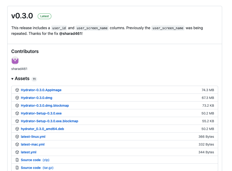
The prebuilt versions of the Hydrator on github.
You will also need a Twitter account to get a Twitter API key, which essentially authorizes you to download tweet data from Twitter. Once you have an account, you can get the key under the Settings on the Hydrator. Doing so will send you to a link asking you to authorize the Hydrator; authorize the app to continue.
After you have authorized the Hydrator, you need to upload the dataset. Under the “Add” menu tab, click “Select Tweet ID File”. This will open your OS file directory where you need to find the unzipped tweet-id file. You can find in in the files you downloaded from TweetSets (if you’re not using TweetSets, you will still need a dehydrated document with a series of Tweet IDs). You can see below that this looks like a series of 18 digit ID numbers, each of which corresponds to a specific tweet on Twitter, and that the Hydrator will link with the tweet itself, along with a bunch of associated metadata.
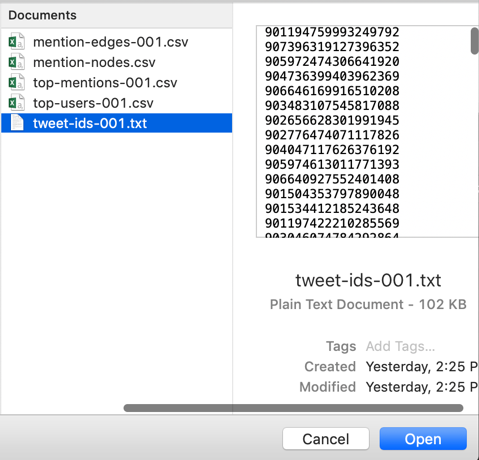
A preview of the dehydrated tweet-ids file.
Once you have found the right file, upload it to the Hydrator.
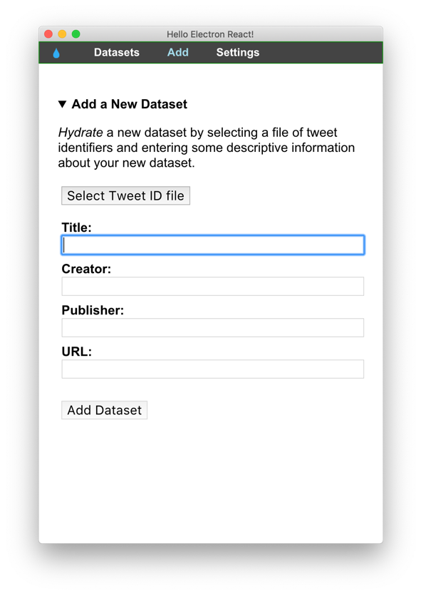
Hydrator prompts for a title and a tweet ID file.

The tweet ID file looks like a series of 18 digit numbers. It’s probably the only .txt file in those you downloaded from TweetSets.
Once you have loaded the Tweet ID file, you should see the file path populate in the Hydrator, as well as an overview of the number of tweets detected.
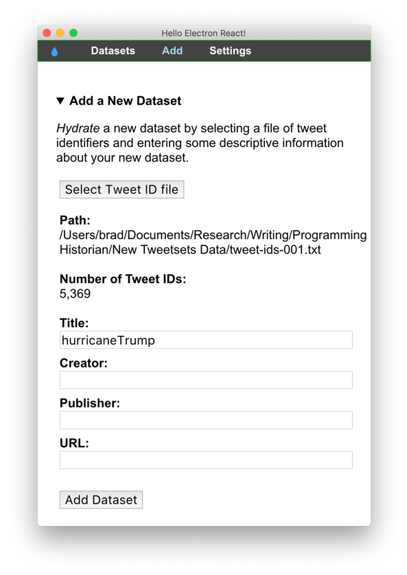
If you’ve loaded your tweet-ID file correctly, Hydrator should display its file path, and the number of tweets in the dataset.
You will need to create a name for your hydrated file, but can ignore the rest of the fields on this screen. Click “Add dataset,” and you will be taken to a screen where you can begin the hydration. To start the hydration, click “Start”. This will prompt another window asking for a name and location to save the hydrated tweets. The program will produce a .json file by default. We’re going to use a .csv format instead to ensure that the file can be easy read by excel or other spreadsheet programs. “CSV” stands for comma-separated values, a non-proprietary file format that uses commas to separate or delimited values in a table. This simple delimiting practice enables a wide variety of programs to translate data in this format. We can do this by clicking on the “CSV” button in the Hydrator after the hydration has completed. Appending “.csv” to the end of the filename you create will also help spreadsheet software recognize and understand the file.
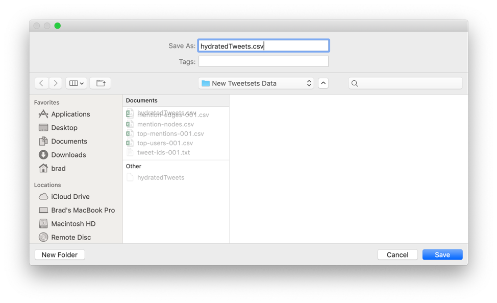
Append .csv to your save file.
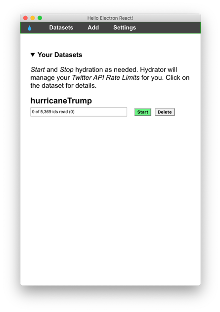
Just press ‘Start’.
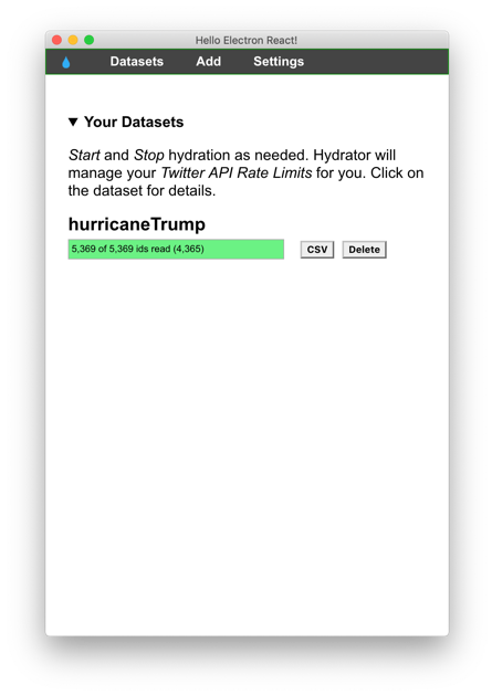
The green bar will fill as your dataset is hydrated.
At this point, your data has gone from the long list of single tweet IDs to a robust, multi-dimensional dataset in .json format. Pressing the “CSV” button will allow you to save it as a CSV instead, which you should do for the purposes of this walkthrough.

The hydrated dataset, blurred here for privacy reasons.
Outputs and How to Use Them
Each tweet now has lots of useful metadata, including the time created, the included hashtags, number of retweets and favorites, and some geo info. One can imagine how this information can be used for a wide variety of explorations, including to map discourse around an issue on social media, explore the relationship between sentiment and virality, or even text analysis of language of the tweets.
All of these processes will probably include some light data work to format this dataset so that you can produce useful insights: statistical analyses, maps, social network analyses, discourse analyses. But regardless of where you go from here, you have a pretty robust dataset that can be used for a variety of academic pursuits.
You might have noticed we didn’t get any latitude/longitude location information, but we did get a “place” column with less exact, textualized location information. Non-coordinate location data needs to be geocoded, which in this case means using a geocoder to geoparse the reported locations and assign lat/long values to them. Different programs do this to greater or lesser success. Tableau, for instance, has a hard time interpolating a set of locations if it’s not at a consistent geographical level (city, state, etc.). For that reason, I generated latitude and longitude information with the Google geocoder following this Programming Historian lesson, and then inputted that information into Tableau for mapping. There’s plenty of good mapping tools out there that you can feel free to use: the key here is getting specific, accurate location information from the list of place names in the dataset.
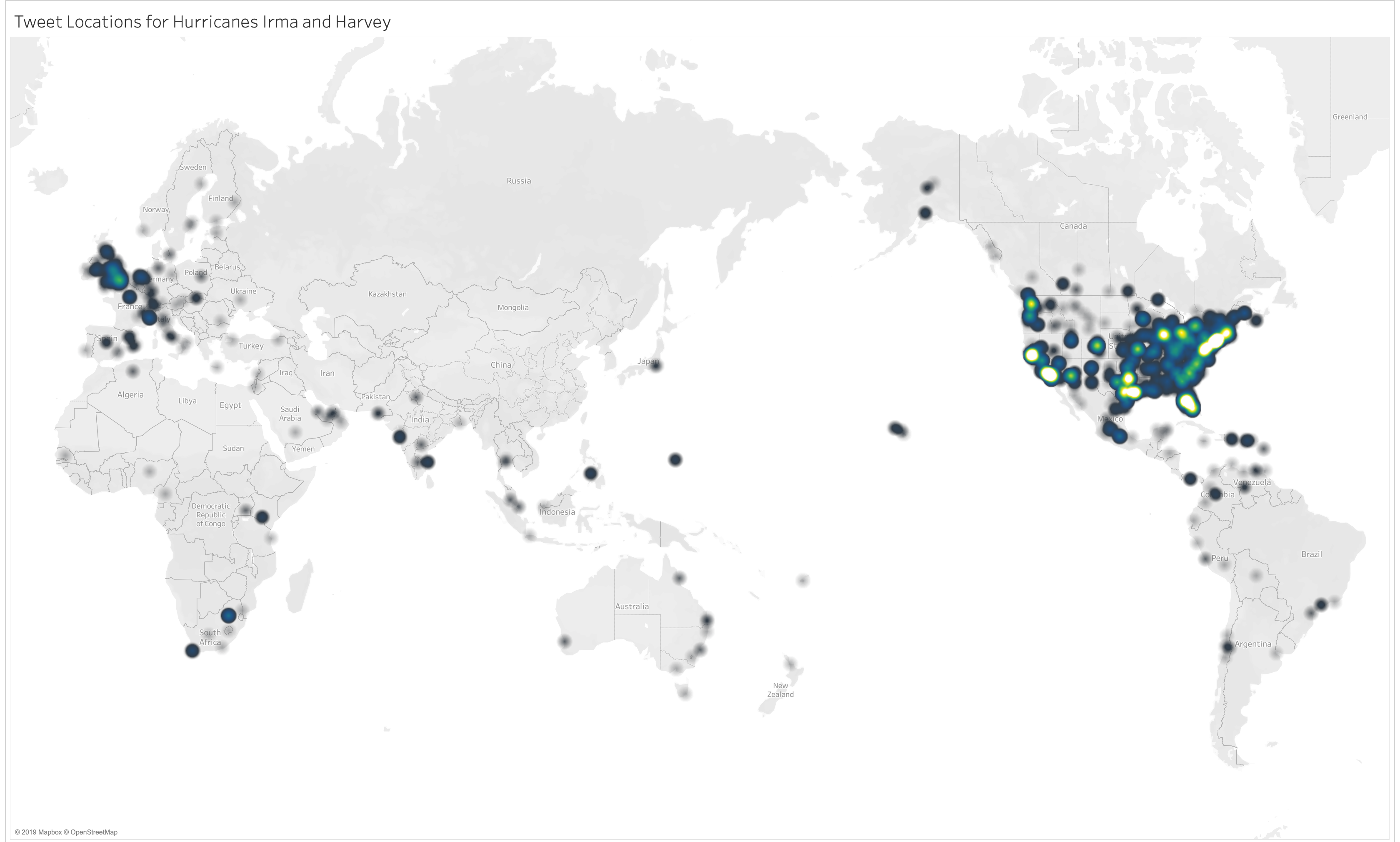
A quick sketch of the "place" data in Tableau. The tweets are taken from just a few days surrounding the storm. One could perhaps argue that these maps show discourse around the storm forming equally in unaffected metro areas as places that fell in the storm’s path.
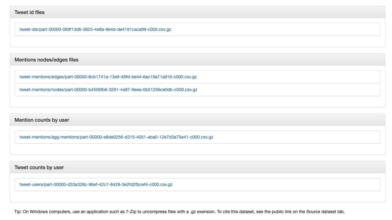
TweetSets provides additional files from the Hurricane Irma dataset. These data files are available for the full dataset only, not our limited subset. To access the files for the full dataset, return to TweetSets and select Hurricane Irma. Do not enter any criteria to limit the dataset (this means all tweets are included). Click Preview and then look at the available files. You can also go directly to the full dataset page. These additional files have some interesting information about the tweets. While the tweet IDs file focuses on specific tweets, the nodes, edges, mentions, and users files give information on how these tweets fit together, and all these files can be correlated to create another robust, linked dataset.
Download and extract the files. On a Windows computer, you can use an application such as 7-Zip to uncompress files with a .gz exension.
If you are unfamiliar with social network analysis, it might be worthwhile to check out one of Scott Weingart’s “Demystifying Networks” series to familiarize yourself with the basic linguistic and visual vocabularies. If you have done so, you will recognize that the TweetSets outputs show us some basic information that can be used to reconstruct a social network. The edges file shows us who is tweeting to whom; the nodes files associates user names with ID numbers; and the top mentions and users files do the same, but for the most actively mentioned and most actively tweeting users.
The edges file is 13,856,080 lines, so too large to work with in Excel. For this lesson, we will work with only the first 1,000 lines of data in the file. The Introduction to the Bash Command Line lesson describes how you can use a command-line interface to read parts of a file using commands such as head. We can read the first 1,001 lines (1,000 lines of data plus a header) of the file into a new file using the following command:
head -1001 edges.csv > edges1000.csv
One Simple (Software Agnostic) Way to Link your Data
At this point, I’m going to cover a very useful data technique that can be employed in a wide variety of spreadsheet platforms (Excel, Google Sheets, Numbers, the open-source Libre Calc), for a wide variety of tasks. I have used it in myriad roles: as a banker, an academic, an administrator, and for personal use. It is called VLOOKUP, which stands for “vertical look up,” and in essence, it makes Excel or other spreadsheet programs function relationally, linking data on unique identifiers. This is not to say that Excel can now be your new SQL, but in limited cases when you need to connect two discrete spreadsheets, it’s an invaluable and easy trick. We’re going to use it to flush out our TweetSets outputs so the data can be used to create a robust and informative social network graph.
When we look at the edges file, we can see it is a series of observations, each consisting of two numbers. These are the ID numbers of Twitter users in this data set: the left column represents the account mentioned and the right one, the “tweeter.” For those familiar with social network analysis (SNA) parlance, these would translate to the “target” and the “source.” At this point, it’s hard to glean much meaningful information from this data, though, as all we have are numbers. VLOOKUP will help with that.
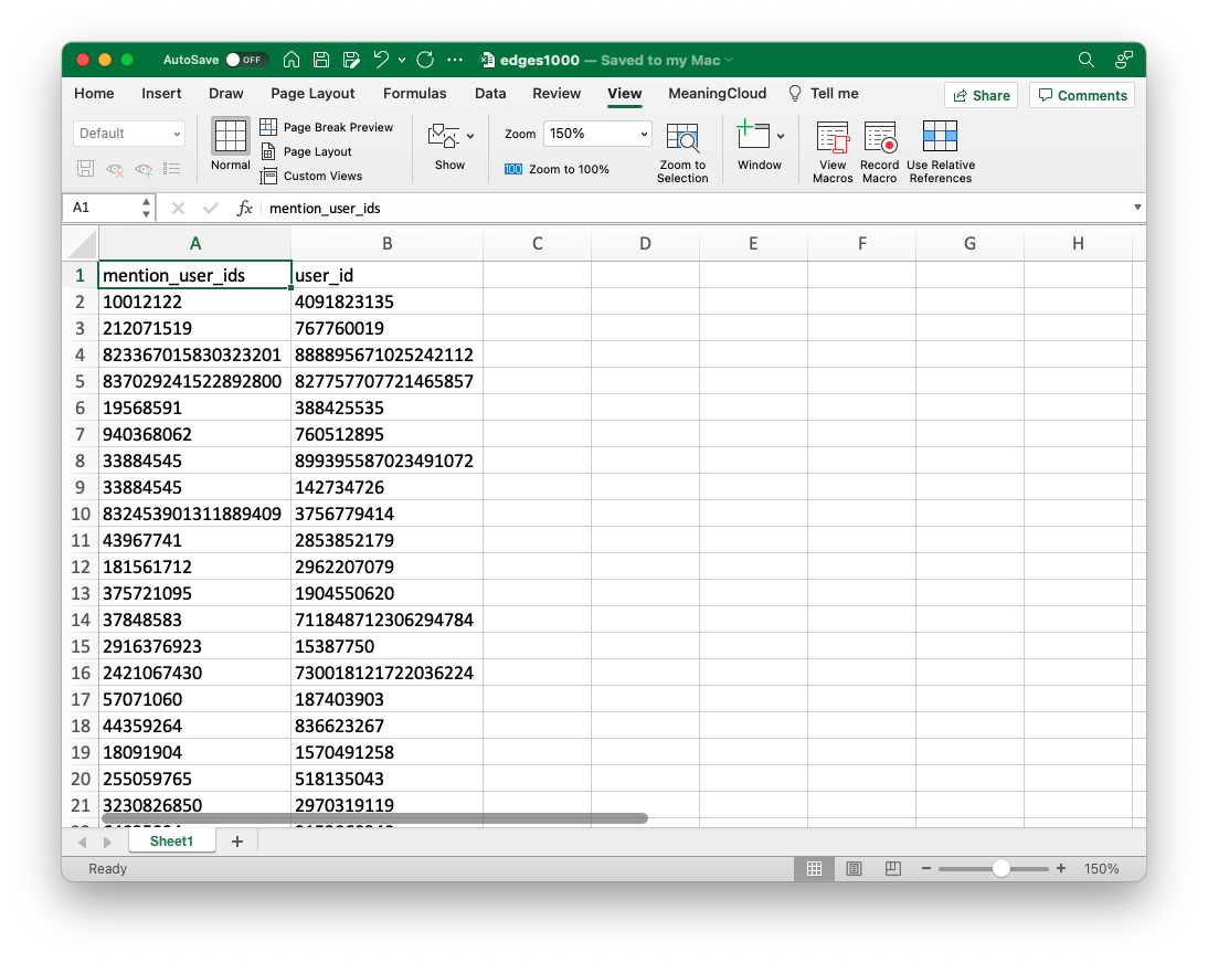
The edges file, preprocessing.
When we open the file (I’ve done it in Excel, but the process is essentially identical in Numbers, Google Sheets, or other spreadsheet programs), it’s possible that some of the longer user IDs have defaulted to scientific notation. We can fix this easily by selecting all the data, going to the format section of the home tab, and selecting “Number.” You might also see that some especially long IDs display as a series of #s. You can also fix this easily by widening the cell, which will allow the full number to display. Finally, the “Decrease Decimal” button, just under the “Number” dropdown, is useful for rendering IDs as whole numbers if they’ve defaulted as decimals. You might run into some of these issues with the other files we’ve downloaded, so keep these solutions in mind.
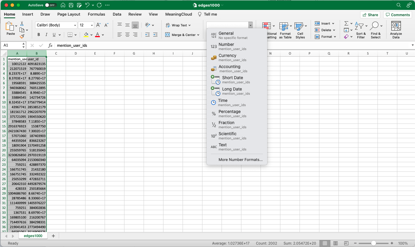
Format the figures as numbers to eliminate scientific notation.
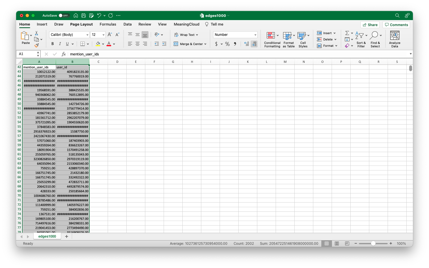
Use "Decrease Decimal" to format the IDs as whole numbers.
Widening the columns will fix the issue of IDs displaying as series of #s.
At this point, we just need to do some quick formatting work to prepare the sheet for the VLOOKUP. Add a column between the two numbers columns so we have space for our additional data to populate. I’ve renamed the columns, “target,” “target_name,” “source,” and “source_name,” loosely following SNA conventions.
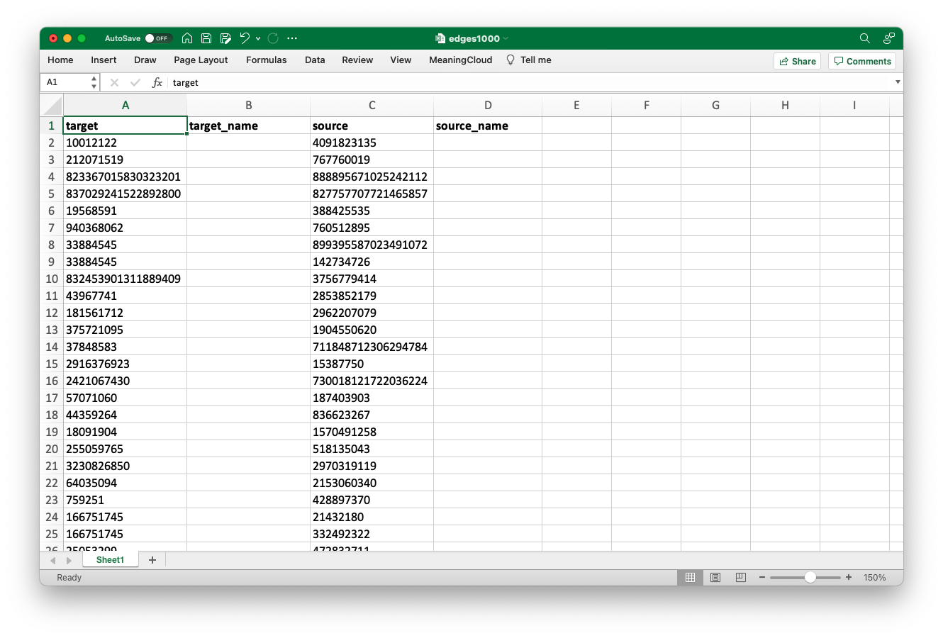
Add a column in the middle and insert the column names above. This will create target cells for the VLOOKUP outputs, and help us keep track of our data.
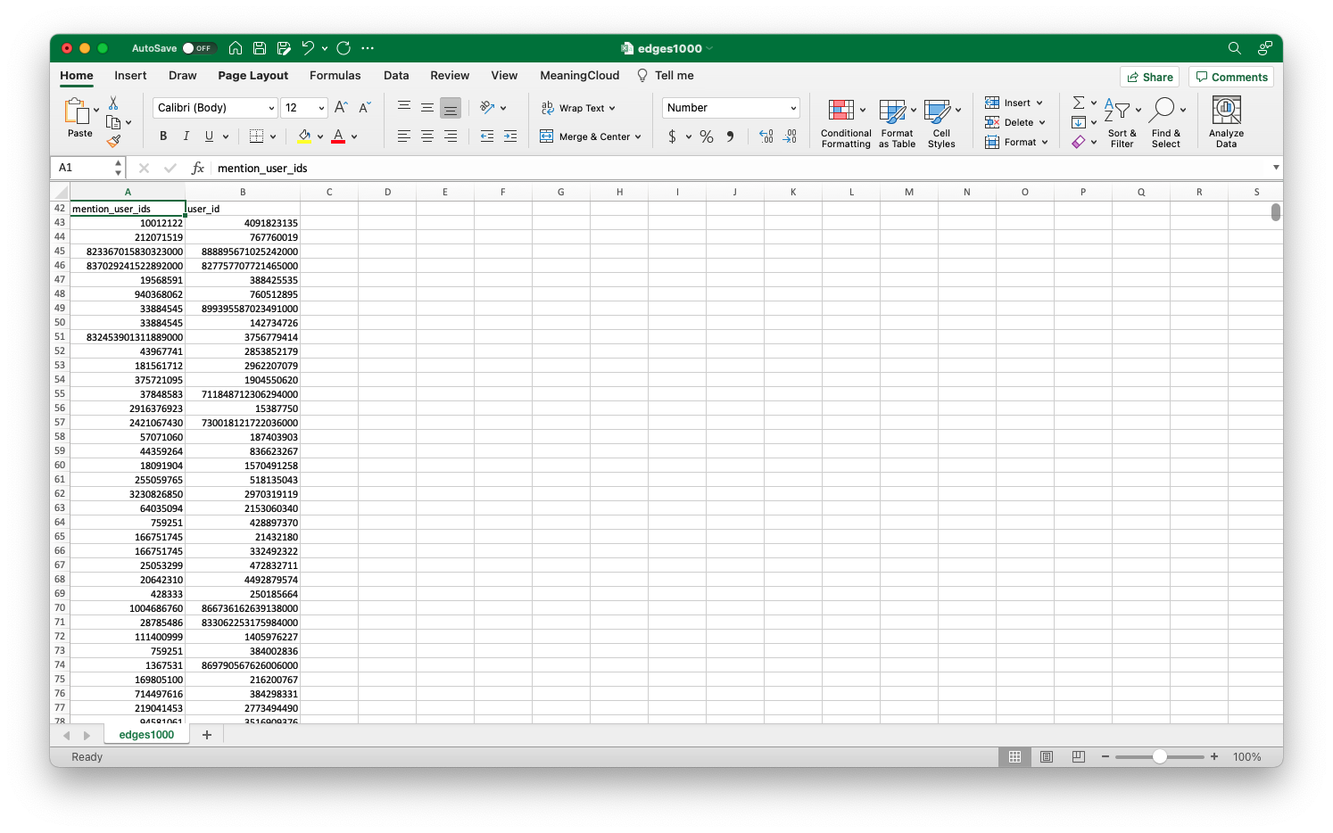
You’ll also want to open the “nodes.csv” spreadsheet at this time. In order for us to use the nodes files in our formula, we need to sort the data by the first column, mention_user_ids. This will allow the VLOOKUP formula to accurately search the column.
Now that everything is formatted, click in the cell to the right of the column on which you want to perform the VLOOKUP. I’m going to start the process with the target column because the people appearing in this column are mostly public figures, enabling me to show you my return values without worrying about privacy issues. You can start with this column or the source column: you’ll perform the process on both.
Once that’s done, we’ll need to search for the VLOOKUP formula. You can also type this out “freehand”, but looking it up will give you access to the Excel (or Sheets or Numbers) formula builder, which makes this task much easier. To do this, go to the “Formulas” tab, click “Insert Function,” and search for “VLOOKUP”.
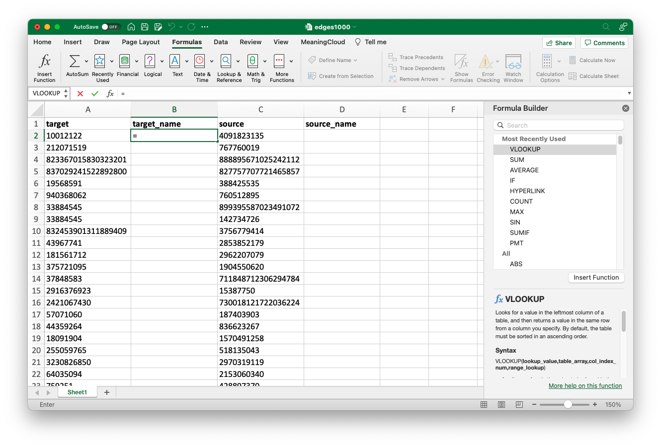
Search for VLOOKUP on the "Formulas" tab.
Once you click on it, you should see a handy formula builder dialog box on the right.
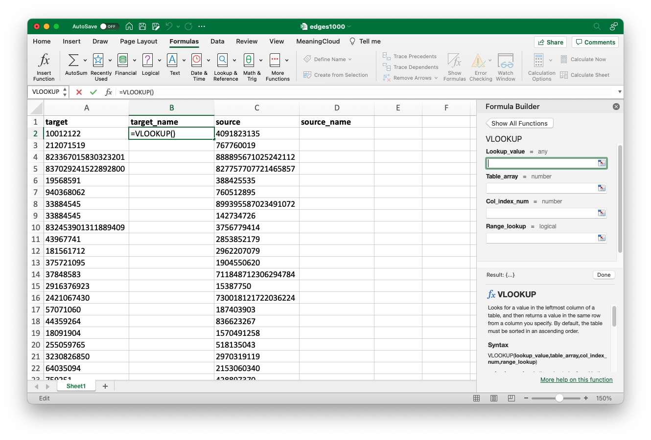
The VLOOKUP formula builder provides fields for input values.
Click in the “Lookup_value” field in the formula builder, then click on the letter at the top of the column of associated ID numbers. Essentially, this input is telling the software the unique ID it will use to link data in two separate spreadsheets. In my case that is column A, so I click on the letter “A” at the top of the column, selecting it in its entirety. You will see the software automatically enters the value “A:A” into the formula builder upon click.
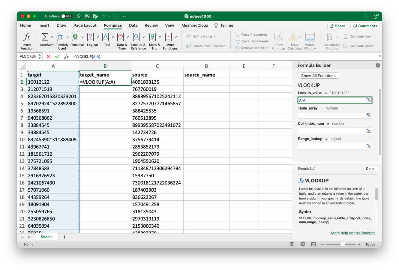
The lookup value is the unique ID you want to match. In this case, it’s the target ID column. You can click on the letter at the top of the column to select it in its entirety.
From here, we’ll move our cursor down to the next dialog box, “Table_array”. This refers to the field of values in the second spreadsheet we want the software to reference when linking our data. Once your cursor is in the dialog box, move over to the second spreadsheet–“nodes.csv” for the target column, “mention_user_ids” for the source–and click and drag to highlight the entire table. For larger datasets, all you need to highlight is the field spanning from the unique ID to the desired return value, but with our smaller dataset, that means the entire spreadsheet. When you click back to the “edges” sheet, you’ll see some complex syntax has populated.
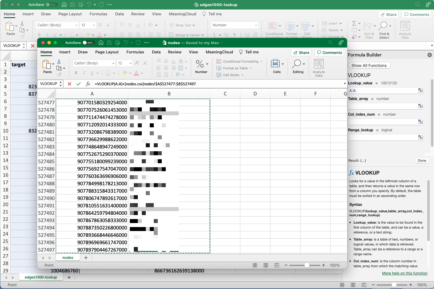
Highlight all the values in the second spreadsheet.
The final two inputs are easy, but I’ll take a moment to explain what they mean. “Col_index_num” tells the software what value you want it to return. We want the target name, which is in the second column of our table array, so we put the number “2”. You’ll need to adjust this as necessary with different datasets. The “range_lookup” field tells the software whether the match for the lookup value needs to be exact. “FALSE” tells it that it does.
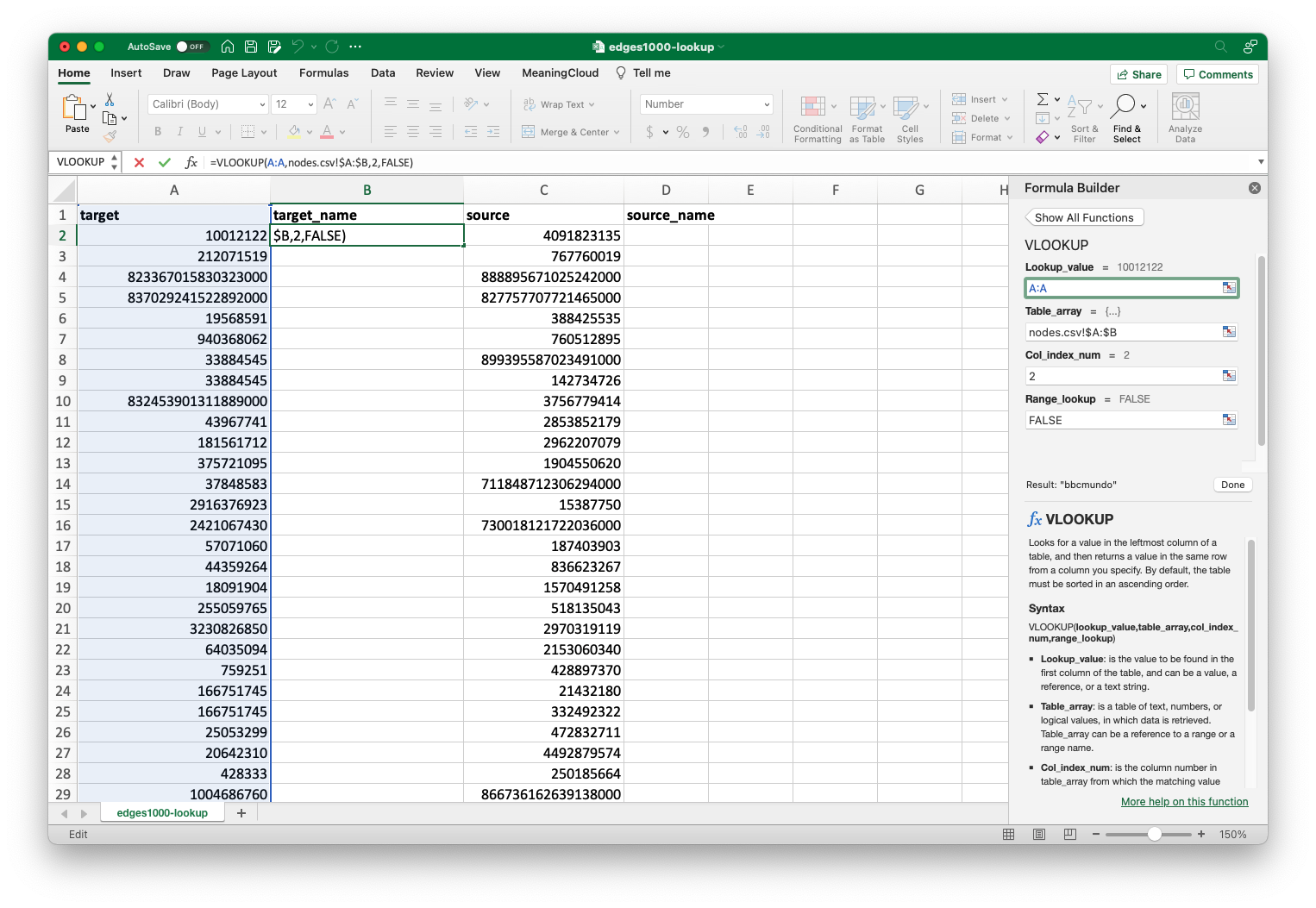
All inputs completed. The "Result" at the bottom near the "Done" button will give you some idea if your inputs were correct. If it looks alright, you can go ahead and click "Done".
When you click “Done”, you will see the first value populate in the cell. If you get an alert saying, “The formula you have entered may spill beyond the edges of the worksheet,” then click Yes to insert the suggested formula. Note that the formula is still displayed in the formula box at the top, not the returned value. We’ll remedy this in a moment. For now, you’ll want to hover over the black box in the lower right hand corner of this cell. Your cursor should change to a black plus sign when you do. From there, click and drag the cell all the way down the column. When you get to the bottom of the sheet, you can release the mouse button, and you should see values populate for all the rows. This may take a while with larger datasets, but it’s pretty quick with this one.
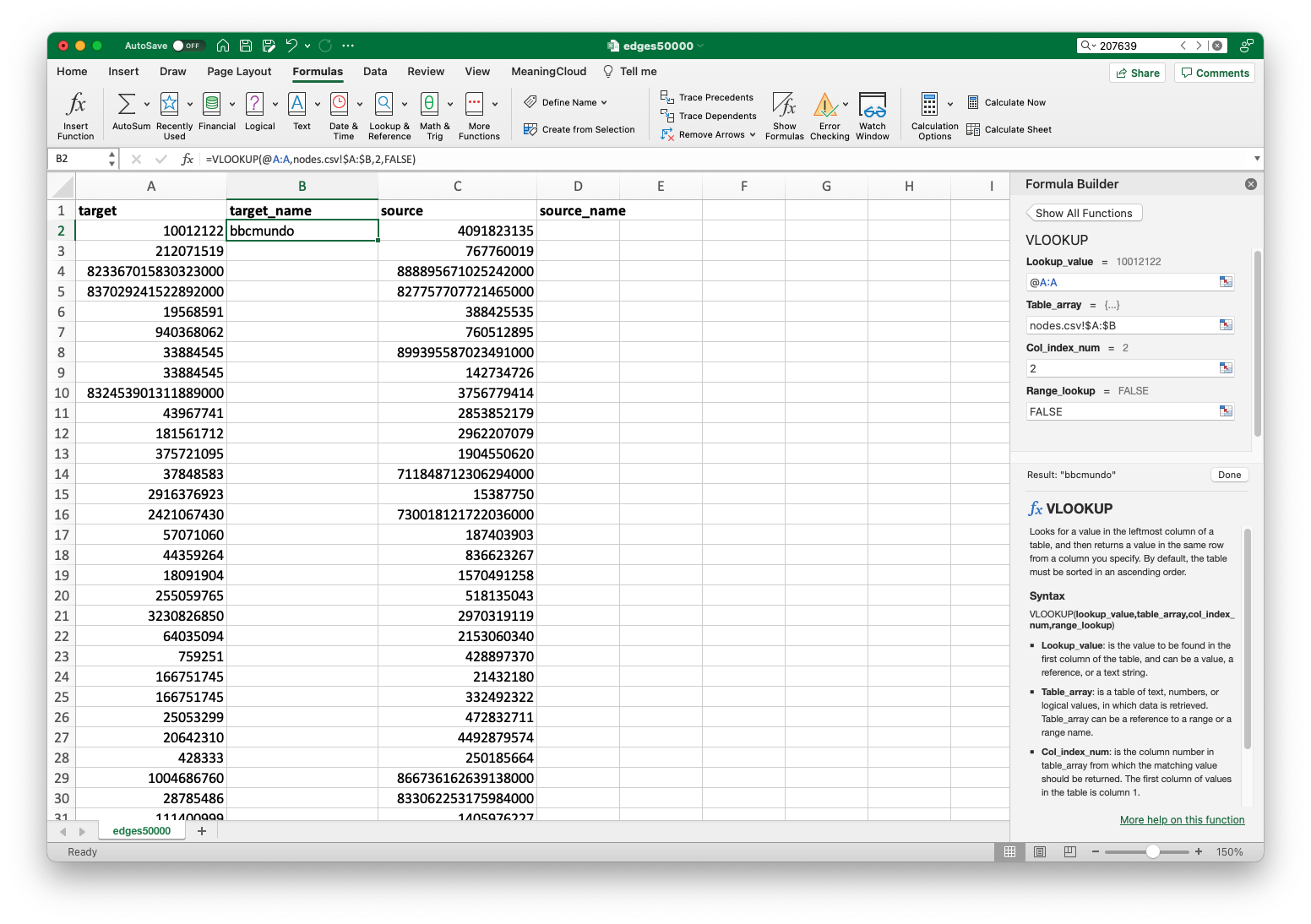
If you’ve done everything correctly, you’ll see a return value in the cell you clicked on earlier, and the formula in the "fx" field.
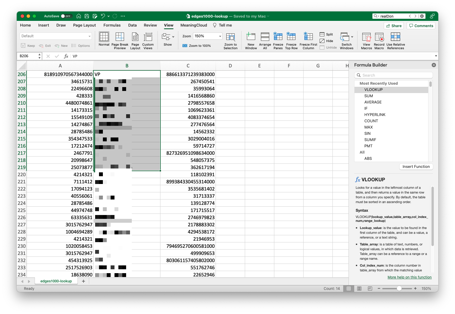
With just a few steps, we now know the real world people associated with each user ID.
You might, however, notice that instead of the usernames we’re interested in, each cell contains the formula we used to retrieve them. This can be an issue if the spreadsheet program ever loses track of the second spreadsheet: if it can’t find it, it won’t be able to return the value in the future. To remedy this, we’re going to paste the returned values into the cells rather than the formula. At this point you should already have the column highlighted, so you can press command + C (ctrl + C on Windows) to copy the column, then right click and select “Paste Special.”
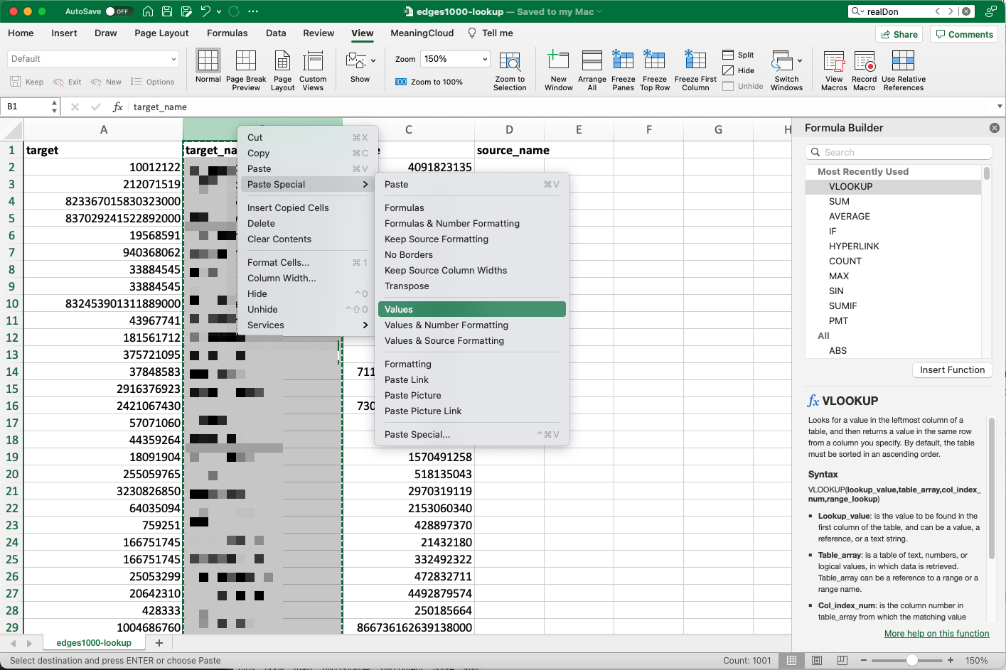
Copy->Paste Special will allow us to tell the software to insert the actual return values, rather than the formula, into the spreadsheet.
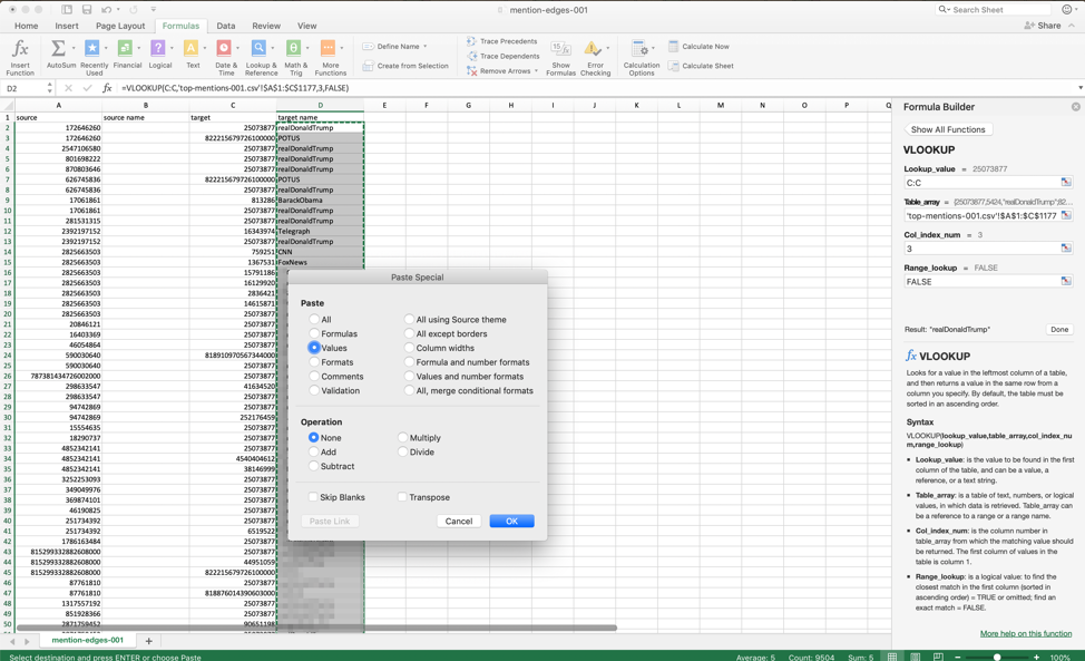
Choose "Values" in the "Paste Special" menu.
Once you’ve done this, you can see the returned value is now in the formula field at the top, rather than the formula. This will prevent the CSV from “breaking” in the future. Though retaining the formula would, in theory, allow the spreadsheet to auto-update in the future, it’s probably easier to just rerun the VLOOKUP, rather than having to make sure the main spreadsheet always knows where the reference spreadsheets are located.
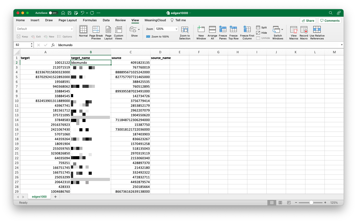
Done with data formatting!
Further Applications
After repeating this process on the second column, this spreadsheet is ready to be used in a variety of social network visualizations. It will drop right in to a SNA tool like Palladio, or, with some light reformatting, into software like Gephi or Cytoscape. The VLOOKUP we did makes it so you can do the visualizations with human-legible user names, rather than rather meaningless user IDs.
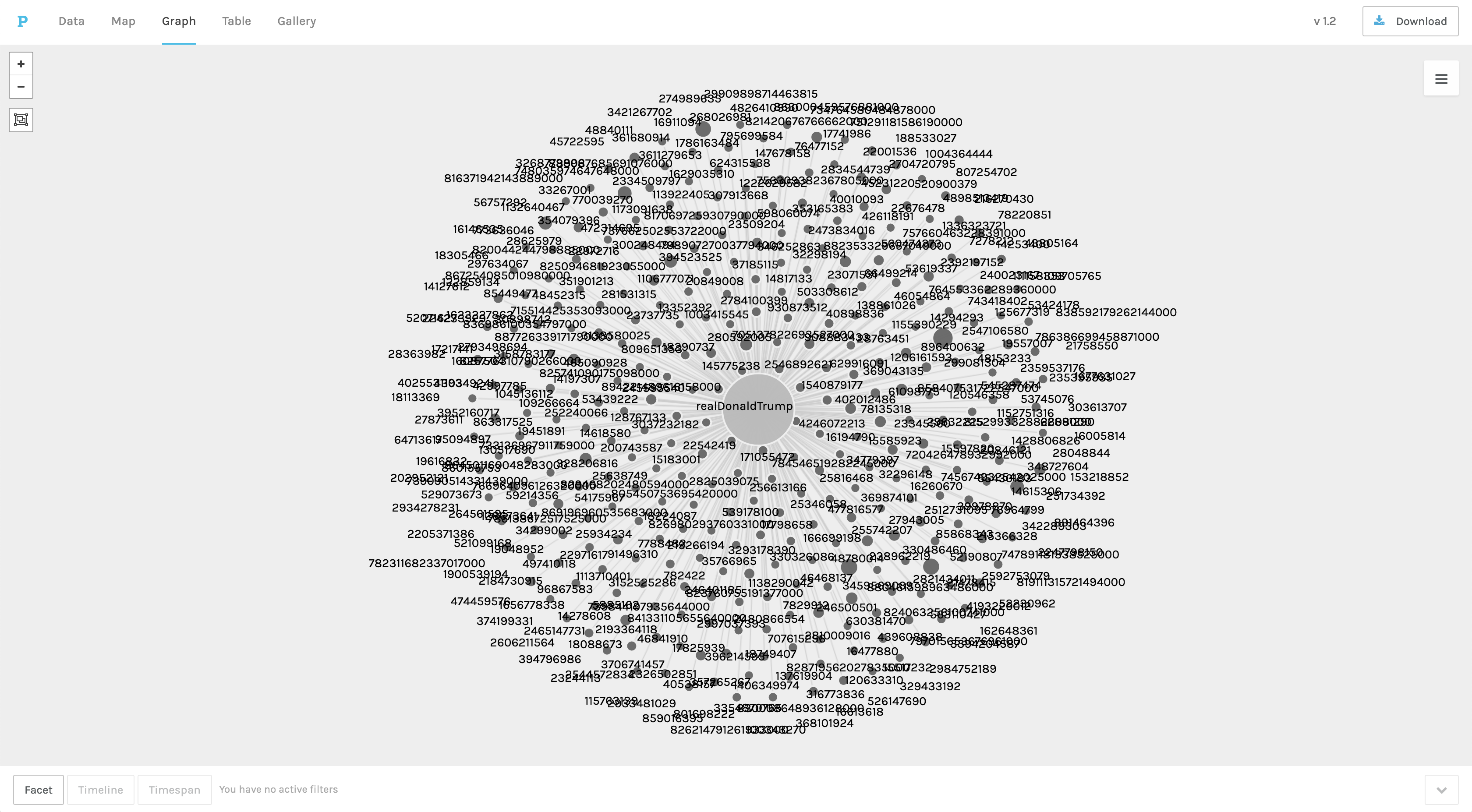
A very quick social network sketch showing the users who most often mentioned @realDonaldTrump in their hurricane tweets. Done in Palladio.
Conclusion
At this point, you have several datasets that will work well in a wide range of digital humanities platforms and methodologies. The hydrated tweet set has qualitative geographic information you can geocode and map, timestamps you can use to build a narrative of a news cycle, tweet text you can on which you can perform natural language or discourse analysis, and other very rich data points for doing historical or civic research.
The nodes and edges information we produced is ready to be used in a wide variety of social networking, but more importantly, you can use the VLOOKUP method for a wide variety of data correlation tasks that might not warrant learning and using something like SQL. I use it all the time in my research to connect file names or unique IDs to more substantive metadata like author names, publication dates, or book titles.
While this tutorial focuses on simplified methods, it should serve as a kind of “on-ramp” to show beginners that digital research–collecting thousands of data points, preparing those data points, and doing some sort of analysis/visualizaiton of them–is within reach. In completing this lesson, you should be able to approximate many of the research results of scholars trained in digital methods, and should be much closer to enacting more advanced methods, should you choose.