Contents
- Introduction
- Some Background on Sonification
- Musicalgorithms
- A quick word about getting Python set up
- MIDITime
- Sonic Pi
- Nihil Novi Sub Sole
- Conclusion
- References
Introduction
ποίησις - fabrication, creation, production
I am too tired of seeing the past. There are any number of guides that will help you visualize that past which cannot be seen, but often we forget what a creative act visualization is. We are perhaps too tied to our screens, too much invested in ‘seeing’. Let me hear something of the past instead.
While there is a deep history and literature on archaeoacoustics and soundscapes that try to capture the sound of a place as it was (see for instance the Virtual St. Paul’s or the work of Jeff Veitch on ancient Ostia), I am interested instead to ’sonify’ what I have right now, the data themselves. I want to figure out a grammar for representing data in sound that is appropriate for history. Drucker famously reminds us that ‘data’ are not really things given, but rather things captured, things transformed: that is to say, ‘capta’. In sonifying data, I literally perform the past in the present, and so the assumptions, the transformations, I make are foregrounded. The resulting aural experience is a literal ‘deformance’ (portmanteau of ‘deform’ and ‘perform’) that makes us hear modern layers of the past in a new way.
I want to hear the meaning of the past, but I know that I can’t. Nevertheless, when I hear an instrument, I can imagine the physicality of the player playing it; in its echoes and resonances I can discern the physical space. I can feel the bass; I can move to the rhythm. The music engages my whole body, my whole imagination. Its associations with sounds, music, and tones I’ve heard before create a deep temporal experience, a system of embodied relationships between myself and the past. Visual? We have had visual representations of the past for so long, we have almost forgotten the artistic and performative aspect of those grammars of expression.
In this tutorial, you will learn to make some noise from your data about the past. The meaning of that noise, well… that’s up to you. Part of the point of this tutorial is to make your data unfamiliar again. By translating it, transcoding it, remediating it, we begin to see elements of the data that our familiarity with visual modes of expression have blinded us to. This deformation, this deformance, is in keeping with arguments made by for instance Mark Sample on breaking things, or Bethany Nowviskie on the ‘resistance in the materials’. Sonification moves us along the continuum from data to capta, social science to art, glitch to aesthetic. So let’s see what this all sounds like.
Objectives
In this tutorial, I will introduce you to three different ways of generating sound or music from your data.
In the first, we will use a freely available and free-to-use system developed by Jonathan Middleton called Musicalgorithms, to introduce some of the issues and key terms involved. In the second, we will use a small python library to ‘parameter map’ our data against the 88 key keyboard, and introduce some artistry into our work. Finally, we will learn how to load our data into the open source live-coding environment for sound and music, Sonic Pi, at which time I will leave you to explore that project’s copious tutorials and resources.
You will see that ‘sonification’ moves us along the spectrum from mere ‘visualization/auralization’ to actual performance.
Tools
- Musicalgorithms http://musicalgorithms.org/
- MIDITime https://github.com/cirlabs/miditime (I have forked a copy here)
- Sonic Pi http://sonic-pi.net/
Example Data
- Roman artefact data
- Excerpt from the Topic model of John Adams’ Diary
- Excerpt from the Topic model of the Jesuit Relations
Some Background on Sonification
Sonification is the practice of mapping aspects of the data to produce sound signals. In general, a technique can be called ‘sonification’ if it meets certain conditions. These include reproducibility (the same data can be transformed the same ways by other researchers and produce the same results) and what might be called intelligibility - that the ‘objective’ elements of the original data are reflected systematically in the resulting sound (see Hermann 2008 for a taxonomy of sonification). Last and Usyskin (2015) designed a series of experiments to determine what kinds of data-analytic tasks could be performed when the data were sonified. Their experimental results (Last and Usyskin 2015) have shown that even untrained listeners (listeners with no formal training in music) can make useful distinctions in the data. They found listeners could discriminate in the sonified data common data exploration tasks such as classification and clustering. (Their sonified outputs mapped the underlying data to the Western musical scale.)
Last and Usyskin focused on time-series data. They argue that time-series data are particularly well suited to sonification because there are natural parallels with musical sound. Music is sequential, it has duration, and it evolves over time; so too with time-series data (Last and Usyskin 2015: 424). It becomes a problem of matching the data to the appropriate sonic outputs. In many applications of sonification, a technique called ‘parameter mapping’ is used to marry aspects of the data along various auditory dimensions such as pitch, variation, brilliance, and onset. The problem with this approach is that where there is no temporal relationship (or rather, no non-linear relationship) between the original data points, the resulting sound can be ‘confusing’ (2015: 422).
Hearing the Gaps
There is also the way that we fill in gaps in the sound with our expectations. Consider this video where the mp3 has been converted to MIDI back to mp3; the music has been ‘flattened’ so that all sonic information is being played by one instrument. (Generating this effect is rather like saving a webpage as .txt, opening it in Word, and then resaving it as .html). All sounds (including vocals) have been translated to their corresponding note values, and then turned back into an mp3.
It is noisy; yet we perceive meaning. Consider the video below:
What’s going on here? If that song was already known to you, you probably heard the actual ‘words’. Yet, no words are present in the song! If the song was not already familiar to you, it sounded like garbled nonsense (see more examples on Andy Baio’s website). This effect is sometimes called an ‘auditory hallucination’(cf. Koebler, 2015). This example shows how in any representation of data we can hear/see what is not, strictly speaking, there. We fill the holes with our own expectations.
Consider the implications for history. If we sonify our data, and begin to hear patterns in the sound, or odd outliers, our cultural expectations about how music works (our memories of similar snippets of music, heard in particular contexts) are going to colour our interpretation. This I would argue is true about all representations of the past, but sonifying is just odd enough to our regular methods that this self-awareness will help us identify or communicate the critical patterns in the (data of the) past.
We will progress through three different tools for sonifying data, noting how choices in one tool affect the output, and can be mitigated by reimagining the data via another tool. Ultimately, there is nothing any more objective in ‘sonification’ than there is in ‘visualization’, and so the investigator has to be prepared to justify her choices, and to make these choices transparent and reproducible for others. (And lest we think that sonification and algorithmically generated music is somehow a ‘new’ thing, I direct the interested reader to Hedges, (1978).)
In each section, I will give a conceptual introduction, followed by a walkthrough using sample archaeological or historical data.
Musicalgorithms
There are a wide variety of tools out there to sonify data. Some for instance are packages for the widely-used R statistical environment, such as ‘playitbyR’ and ‘AudiolyzR’. The first of these however has not been maintained or updated to work with the current version of R (its last update was a number of years ago), and the second requires considerable configuration of extra software to make it work properly.
By contrast, the Musicalgorithms site is quite easy to use. The Musicalgorithms site has been online for over a decade. Though it is not open source, it represents a long-term research project in computational music by its creator, Jonathan Middleton. It is currently in its third major iteration (earlier iterations remain usable online). We will begin with Musicalalgorithms because it allows us to quickly enter and tweak our data to produce a MIDI file representation. Make sure to select ‘Version 3.’
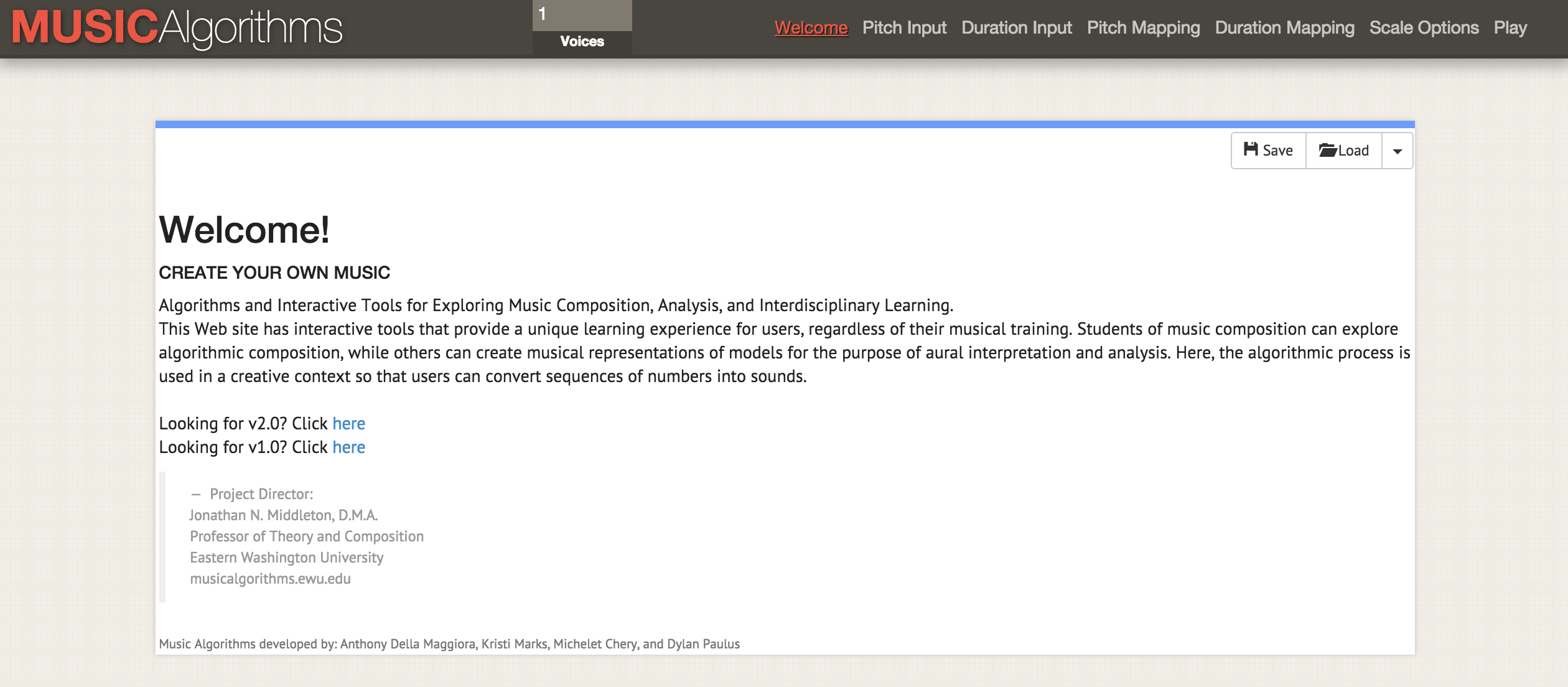
The Musicalgorithms Website as it appeared on February 2nd, 2016
Musicalgorithms effects a number of transformations on the data. In the sample data below (the default from the site itself), there is but one row of data, even if it looks like several rows. The sample data is comprised of comma separated fields that are themselves space delimited.
# Of Voices, Text Area Name, Text Area Data
1,morphBox,
,areaPitch1,2 7 1 8 2 8 1 8 2 8 4 5 9 0 4 5 2 3 5 3 6 0 2 8
,dAreaMap1,2 7 1 8 2 8 1 8 2 8 4 5 9 0 4 5 2 3 5 3 6 0 2 8
,mapArea1,20 69 11 78 20 78 11 78 20 78 40 49 88 1 40 49 20 30 49 30 59 1 20 78
,dMapArea1,1 5 1 5 1 5 1 5 1 5 3 3 6 0 3 3 1 2 3 2 4 0 1 5
,so_text_area1,20 69 11 78 20 78 11 78 20 78 40 49 88 1 40 49 20 30 49 30 59 1 20 78
This data represents the source data and its transformations; sharing this data would allow another investigator to replicate or extend the sonification using other tools. When one begins however, only the basic data below is needed (a list of data points):
# Of Voices, Text Area Name, Text Area Data
1,morphBox,
,areaPitch1,24 72 12 84 21 81 14 81 24 81 44 51 94 01 44 51 24 31 5 43 61 04 21 81
The key field for us is ‘areaPitch1,’ which contains the space-delimited input data. The other fields will become filled as we move through Musicalgorithms’ various settings. In the data above (eg 24 72 12 84 etc), the values are raw counts of inscriptions from a series of sites along a Roman road in Britain. (We will practice with other data in a moment below).
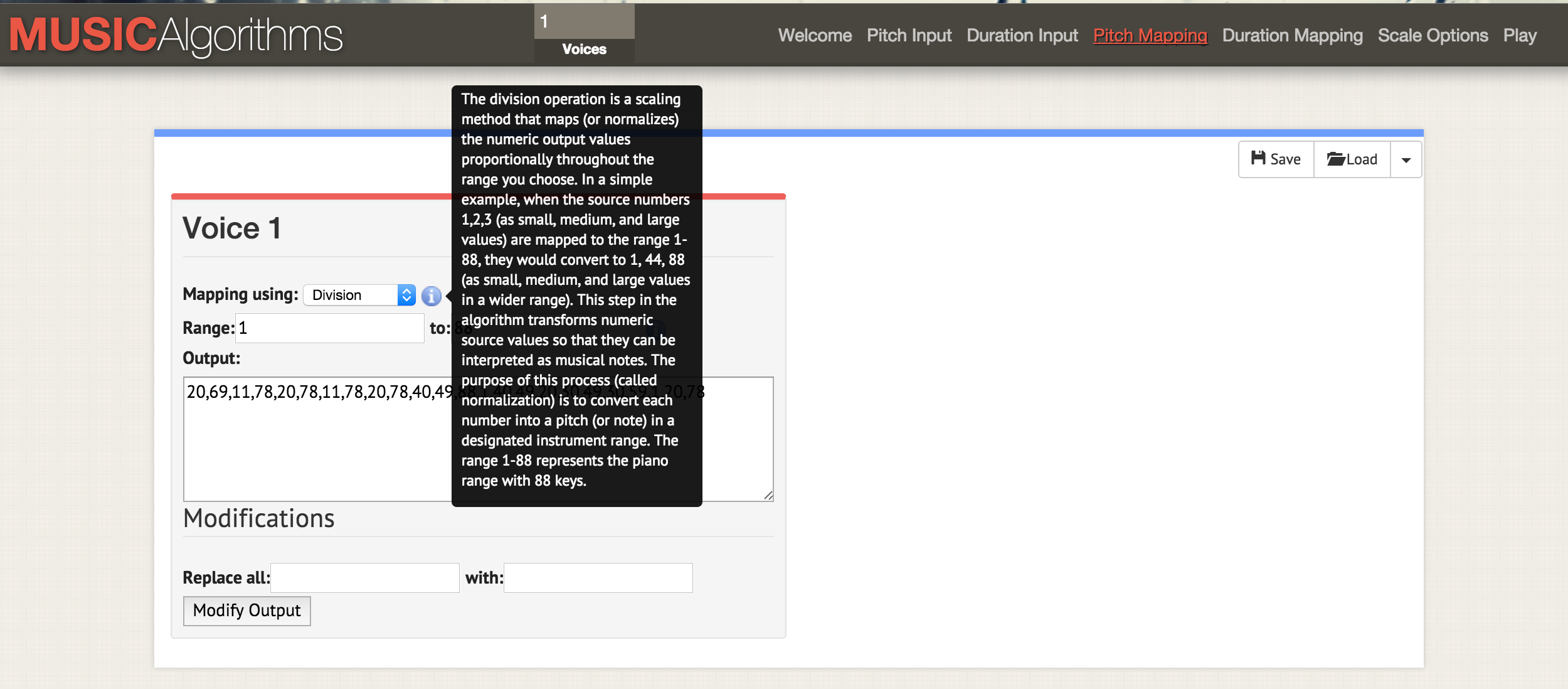
After you load your data, you can select the different operations across the top menu bar of the site. In the screenshot, the information mouseover is explaining what happens to the scaling of your data if you select the division operation to scale your data to the range of notes selected.
Now, as you page across the various tabs in the interface (‘duration input’, ‘pitch mapping’, ‘duration mapping’, ‘scale options’) you can effect various transformations. In ‘pitch mapping’, there are a number of mathematical options for mapping the data against the full 88 keys/pitches of a piano keyboard (in a linear mapping, the mean of one’s data would be mapped to middle C, or 40). One can also choose the kind of scale, whether it is a minor or major and so on. At this point, once you’ve selected your various transformations, you should save the text file. On the file tab, ‘play’, one can download a midi file. Your default audio program can play midi files (often defaulting to a piano tone). More complicated instrumentation can be assigned by opening the midi file in music mixing programs such as GarageBand (Mac) or LMMS (Windows, Mac, Linux). (Using Garageband or LMMS are outside the scope of this tutorial. A video tutorial on LMMS is available here, while Garageband tutorials proliferate online. Lynda.com has an excellent one)
If you had several columns of data for the same points - say, in our example from Roman Britain, we also wanted to sonify counts of a pottery type for those same towns - you can reload your next data series, effect the transformations and mappings, and generate another MIDI file. Since Garageband and LMMS allow for overlaying of voices, you can begin to build up complicated sequences of music.
.](/images/sonification/sonification-garageband-john-adams-3.png)
Screenshot of Garageband, where the midi files are sonified topics from John Adams’ Diary. In the Garageband interface (LMMS is similar), each midi file is dragged-and-dropped into place. The instrumentation for each midi file (ie track) can be selected from Garageband’s menus. The labels for each track have here been changed to reflect the key words in each topic. The green area to the right represents a visualization of the notes in each track. You can watch this interface in action and listen to the music here.
Which transformations should you use? If you had two columns of data, you have two voices. It might make sense, in our hypothetical data, to play the first voice loud, in a major key: inscriptions ‘speak’ to us, in a manner of speaking, after all. (Roman inscriptions do address the reader, the passerby, literally: ‘O you who passes by…’). Then, perhaps since the pottery you are interested in are humble wares, perhaps they would be mapped against the lower end of the scale, or given longer duration notes to represent their ubiquity across classes in this region.
There is no ‘right’ way to represent your data as sound, at least not yet: but even with this simple example, we begin to see how shades of meaning and interpretation can be inflected into our data and into our experience of that data.
But what about time? Historical data often has a punctuation point, a distinct ‘time when’ something occured. Thus, the amount of time between two data points has to be taken into account. This is where our next tool becomes quite useful, for when our data points have a relationship to one another in temporal space. We begin to move from sonfication (data points) to music (relationships between points).
Practice
The sample dataset provided contains counts of Roman coins in its first column and counts of other Roman materials from the same locations, as contained in the Portable Antiquities Scheme database from the British Museum. A sonification of this data might reveal or highlight aspects of the economic situation along Watling street, a major route through Roman Britain. The data points are organized geographically from North West to South East; thus as the sound plays out, we are hearing movement over space. Each note represents another stop along the way.
- Open thesonification-roman-data.csv in a spreadsheet. Copy the first column into a text editor. Delete the line endings so that the data is all in a single row.
- Add the following column information like so:
# Of Voices, Text Area Name, Text Area Data
1,morphBox,
,areaPitch1,
…so that your data follows immediately after that last comma (as like this). Save the file with a useful name like
coinsounds1.csv. - Go to the Musicalgorithms site (version 3), and hit the load button. In the pop-up, click the blue ‘load’ button and select the file saved in step 2. The site will load your materials and display a green check mark if it loaded successfully. If it did not, make sure that your values are separated by spaces, and that they follow immediately the last comma in the code block in step 2. You may also try loading up the demo file for this tutorial instead.
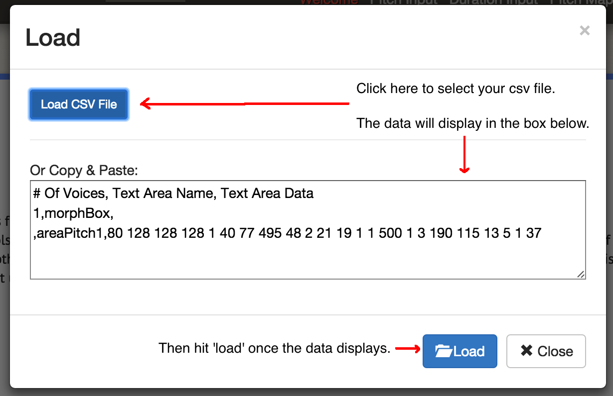
Click ‘load’ on the main screen to get this dialogue box. Then ‘load csv’. Select your file; it will appear in the box. Then click the bottom load button.
- Click on ‘Pitch Input’. You’ll see the values of your data. For now, do not select any further options on this page (thus using the site’s default values).
- Click on ‘Duration Input’. Do not select any options here for now. The options here will map various transformations against your data that will alter the duration for each note. Do not worry about these options for now; move on.
- Click on ‘Pitch Mapping’. This is the most crucial choice, as it will transform (that is, scale) your raw data to a mapping against the keys of the keyboard. Leave the
mappingset to ‘division’. (The other options are modulo or logarithmic). The optionRange1 to 88 uses the full 88 keys of the keyboard; thus your lowest value would accord to the deepest note on the piano and your highest value with the highest note. You might wish instead to constrain your music around middle C, so enter 25 to 60 as your range. The output should change to:31,34,34,34,25,28,30,60,28,25,26,26,25,25,60,25,25,38,33,26,25,25,25These are no longer your counts; they are notes on the keyboard.
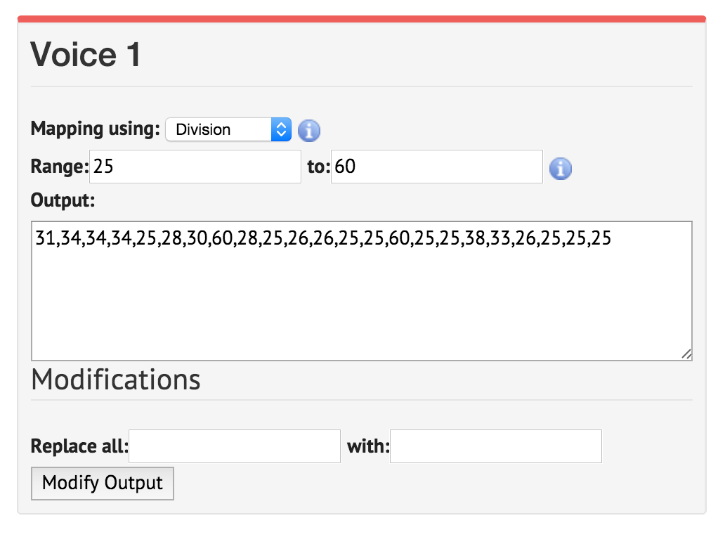
Click into the ‘range’ box and set it to 25. The values underneath will change automatically. Click into the ‘to’ box and set it to 60. Click back into the other box; the values will update.
- Click on ‘Duration Mapping’. Like Pitch Mapping, this takes a range of times that you specify and uses the various mathematical options to map that range of possibilities against your notes. If you mouse over the
iyou will see how the numbers correspond with whole notes, quarter notes, eigth notes, and so on. Leave the default values for now. - Click on ‘Scale Options’. Here we can begin to select something of what might be called the ‘emotional’ aspect to sound. We commonly think of major scales being ‘happy’ while minor scales are ‘sad’; for an accessible discussion see this blog post. For now, select ‘scale by: major’. Leave the ‘scale’ as
C.
You have now sonified one column of data! Click on the ‘save’ button, then ‘save csv’.
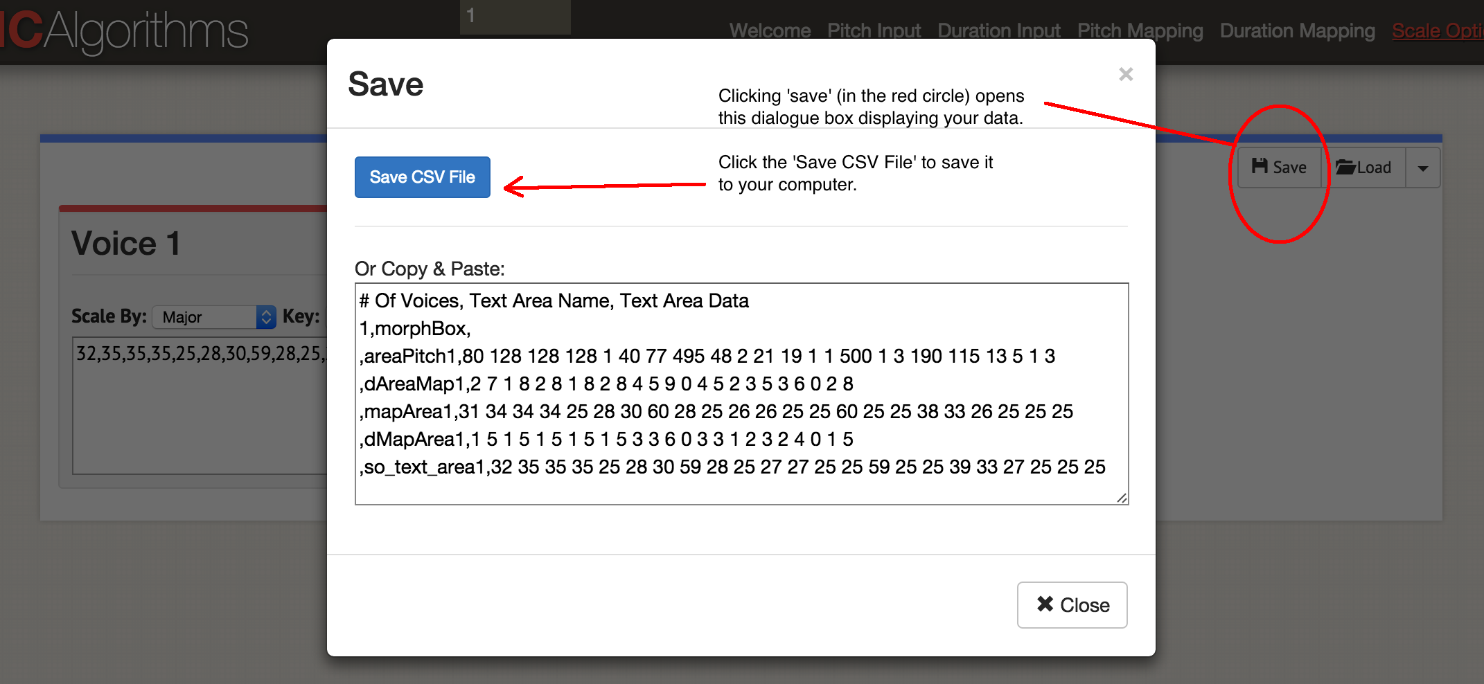
The save data dialogue box.
You’ll have a file that looks something like this:
# Of Voices, Text Area Name, Text Area Data
1,morphBox,
,areaPitch1,80 128 128 128 1 40 77 495 48 2 21 19 1 1 500 1 3 190 115 13 5 1 3
,dAreaMap1,2 7 1 8 2 8 1 8 2 8 4 5 9 0 4 5 2 3 5 3 6 0 2
,mapArea1,31 34 34 34 25 28 30 60 28 25 26 26 25 25 60 25 25 38 33 26 25 25 25
,dMapArea1,1 5 1 5 1 5 1 5 1 5 3 3 6 0 3 3 1 2 3 2 4 0 1
,so_text_area1,32 35 35 35 25 28 30 59 28 25 27 27 25 25 59 25 25 39 33 27 25 25 25
You can see your original data in the ‘areaPitch1’ field, and your subsequent mappings. The site allows you to generate up to four voices at a time into a single MIDI file; depending on how you want to add instrumentation subsequently, you might wish to generate one MIDI file at a time. Let’s play the music - click on ‘Play’. You can select the tempo here, and an instrument. You can listen to your data in the browser, or save as a MIDI file by clicking the blue ‘Save MIDI file’.
Go back to the beginning, and load both columns of data into this template:
# Of Voices, Text Area Name, Text Area Data
2,morphBox,
,areaPitch1,
,areaPitch2,
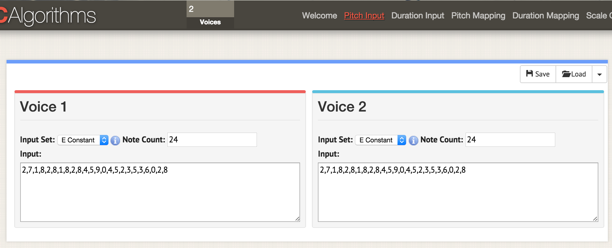
Put 2 into the voices box at the top of the interface. When you then go to any of the option pages - here, we’re at ‘pitch input’ - two displays open up to show you the data for two voices. Load your csv data as before, but have your csv formatted to have ‘areaPitch1’ and ‘areaPitch2’ as described in the main text. The data for voice one will appear on the left, and for voice two on the right.
When you have multiple voices of data, what stands out? Note that in this approach, the distance between points in the real world is not factored into our sonification. This distance, if it were, might be crucical. Distance, of course, does not have to be geographic - it can be temporal. The next tool we’ll explore allows us to factor that into our sonification explicitly.
A quick word about getting Python set up
The next section of this tutorial requires Python. If you haven’t experimented with Python yet, you will need to spend some time becoming familiar with the command line (PC) or terminal (OS). You might find this quick guide to installing python ‘modules’ handy (but come back to it after you read the rest of this section).
Mac users will already have Python installed on their machine. You can test this by holding down the COMMAND button and the spacebar; in the search window, type terminal and click on the terminal application. At the prompt, eg, the cursor blinking at $ type python --version and the computer will respond with what version of python you have. This next section of the tutorial assumes Python 2.7; it has not been tested on Python 3.
For Windows users, Python is not installed by default on your machine so this page will help you get started, though things are a bit more complicated than that page makes out. First, download the .msi file that that page recommends (Python 2.7). Double click the file, and it should install itself in a new directory, eg C:\Python27\. Then, we have to tell Windows the location of where to look for Python whenever you run a python program; that is, you put the location of that directory into your ‘path’, or the environment variable that windows always checks when confronted with a new command. There are a couple ways of doing this, but perhaps the easiest is to search your computer for the program Powershell (type ‘powershell’ into your windows computer search). Open Powershell, and at the > prompt, paste this entire line:
[Environment]::SetEnvironmentVariable("Path", "$env:Path;C:\Python27\;C:\Python27\Scripts\", "User")
You can close powershell when you’re done. You’ll know it worked if nothing very much happens once you’ve pressed ‘enter’. To test that everything is okay, open a command prompt (here are 10 ways to do this) and type at the > prompt python --version. It should tell you Python 2.7.10 or similar.
The last piece of the puzzle that all users will need is a program called Pip. Mac users can install it by typing at the terminal :sudo easy_install pip. Windows users have a bit of a harder time. First, right-click and save-as this link: https://bootstrap.pypa.io/get-pip.py (If you just click on the link, it will show you the code in your browser). Save it somewhere handy. Open a command prompt in the directory where you saved get-pip.py. Then, type at the command prompt python get-pip.py. Conventionally, in tutorials, you will see > or $ at points where you are required to enter something at the command prompt or the terminal. You don’t ever have to type those two characters.
Finally, when you have python code you want to run, you can enter it in your text editor and save it with the .py extension. Your file is a text file, but the file extension tells your computer to use Python to interpret it; but remember, type python at the prompt first, eg: $ python my-cool-script.py.
MIDITime
MIDITime is a python package developed by Reveal News (formerly, the Centre for Investigative Reporting). Its Github repository is here. Miditime is built explicitly for time series data (that is, a sequence of observations collected over time).
While the Musicalgorithms tool has a more-or-less intuitive interface, the investigator sacrifices the ability to know what, exactly, is going on under the hood. In principle, one could examine the underlying code for the MIDITime package to see exactly what’s going on. More importantly, the previous tool had no ability to account for data where the points are distant from one another in clock-time. MIDITime lets us take into account that our data might be clustering in time.
Let us assume that you have a historic diary to which you’ve fitted a topic model. The resulting output might have diary entries as rows, and the percentage composition each topic contributes to that entry as the columns. In which case, listening to these values might help you understand the patterns of thought in the diary in a way that visualizing as a graph might not. Outliers or recurrent musical patterns could stand out to the ear in a way the grammar of graphs obscures.
Installing MIDITime
Installing miditime is straightforward using pip:
$ pip install miditime or $ sudo pip install miditime for a Mac or Linux machine;
> python pip install miditime on a Windows machine. (Windows users, if the instructions above didn’t quite work for you, you might want to try this helper program instead to get Pip working properly on your machine).
Practice
Let us look at the sample script provided. Open your text editor, and copy and paste the sample script in:
#!/usr/bin/python

from miditime.miditime import MIDITime
# NOTE: this import works at least as of v1.1.3; for older versions or forks of miditime, you may need to use
# from miditime.MIDITime import MIDITime

# Instantiate the class with a tempo (120bpm is the default) and an output file destination.
mymidi = MIDITime(120, 'myfile.mid')

# Create a list of notes. Each note is a list: [time, pitch, attack, duration]
midinotes = [
    [0, 60, 200, 3],  #At 0 beats (the start), Middle C with attack 200, for 3 beats
    [10, 61, 200, 4]  #At 10 beats (12 seconds from start), C#5 with attack 200, for 4 beats
]

# Add a track with those notes
mymidi.add_track(midinotes)

# Output the .mid file
mymidi.save_midi()
Save this script as music1.py. At your terminal or command prompt, run the script:
$ python music1.py
A new file, myfile.mid will be written to your directory. To hear this file, you can open it with Quicktime or Windows Media Player. (You can add instrumentation to it by opening it in Garageband or LMMS).
Music1.py imports miditime (remember, you must do pip install miditime before running the script). Then, it creates an output file destination and sets the tempo. The notes are all listed individually, where the first number is the time when the note should be played, the pitch of the note (ie, the actual note!), how hard or rythmically the note is hit (the attack), and then how long the note lasts. The notes are then written to the track, and then the track is written to myfile.mid.
Play with this script now, and add more notes. The notes for ‘Baa Baa Black Sheep’ are:
D, D, A, A, B, B, B, B, A
Baa, Baa, black, sheep, have, you, any, wool?
Can you make your computer play this song? (This chart will help).
By the way There is a text file specification for describing music called ‘ABC Notation’. It is beyond us for now, but one could write a sonification script in say a spreadsheet, mapping values to note names in the ABC specification (if you’ve ever used an IF - THEN in Excel to convert percentage grades to letter grades, you’ll have a sense of how this might be done) and then using a site like this one to convert the ABC notation into a .mid file.
Getting your own data in
This file is a selection from the topic model fitted to John Adams’ Diaries forThe Macroscope. Only the strongest signals have been preserved by rounding the values in the columns to two decimal places (remembering that .25 for instance would indicate that that topic is contributing to a quarter of that diary entry’s composition). To get this data into your python script, it has to be formatted in a particular away. The tricky bit is getting the date field right.
For the purposes of this tutorial, we are going to leave the names of variables and so on unchanged from the sample script. The sample script was developed with earthquake data in mind; so where it says ‘magnitude’ we can think of it as equating to ‘% topic composition.’
my_data = [
    {'event_date': <datetime object>, 'magnitude': 3.4},
    {'event_date': <datetime object>, 'magnitude': 3.2},
    {'event_date': <datetime object>, 'magnitude': 3.6},
    {'event_date': <datetime object>, 'magnitude': 3.0},
    {'event_date': <datetime object>, 'magnitude': 5.6},
    {'event_date': <datetime object>, 'magnitude': 4.0}
]
One could approach the problem of getting our data into that format using regular expressions; it might be easier to just open our topic model in a spreadsheet. Copy the topic data to a new sheet, and leave columns to the left and to the right of the data. In the example below, I put it in column D, and then filled in the rest of the data around it, like so:
| A | B | C | D | E | |
|---|---|---|---|---|---|
| 1 | {‘event_date’: datetime | (1753,6,8) | , ‘magnitude’: | 0.0024499630 | }, |
| 2 | |||||
| 3 |
Then copy and paste the elements that do not change to fill up the entire column. The date element has to be (year,month,day). Once you’ve filled up the table, you can copy and paste it into your text editor so that it becomes part of the my_data array, like so:
my_data = [
{'event_date': datetime(1753,6,8), 'magnitude':0.0024499630},
{'event_date': datetime(1753,6,9), 'magnitude':0.0035766320},
{'event_date': datetime(1753,6,10), 'magnitude':0.0022171550},
{'event_date': datetime(1753,6,11), 'magnitude':0.0033220150},
{'event_date': datetime(1753,6,12), 'magnitude':0.0046445900},
{'event_date': datetime(1753,6,13), 'magnitude':0.0035766320},
{'event_date': datetime(1753,6,14), 'magnitude':0.0042241550}
]
Note that the last row does not have a comma at the end of the line.
Your final script will look something like this, using the example from the Miditime page itself (the code sections below have been interrupted by commentary, but should be pasted into your text editor as a single file):
from miditime.MIDITime import MIDITime
from datetime import datetime
import random

mymidi = MIDITime(108, 'johnadams1.mid', 3, 4, 1)
The values after MIDITime, MIDITime(108, 'johnadams1.mid', 3, 4, 1) set
- the beats per minute (108),
- the output file (‘johnadams1.mid’),
- the number of seconds to represent a year in the music (3 seconds to a calendar year, so all of the notes for diary entries from 1753 will be scaled against 3 seconds; there are 50 years in the data, so the final song will be 50 x 3 seconds long, or a bit over two minutes),
- the base octave for the music (middle C is conventionally represented as C5, so here 4 represents one octave below middle C),
- and how many octaves to map the pitches against.
Now we pass our data into the script by feeding it into the my_data array (this gets pasted in next):
my_data = [
{'event_date': datetime(1753,6,8), 'magnitude':0.0024499630},
{'event_date': datetime(1753,6,9), 'magnitude':0.0035766320},
…have your data in here, remembering to end the final event_date line without a comma, and finishing the data with a ] on its own line, eg
{'event_date': datetime(1753,6,14), 'magnitude':0.0042241550}
]
and then paste:
my_data_epoched = [{'days_since_epoch': mymidi.days_since_epoch(d['event_date']), 'magnitude': d['magnitude']} for d in my_data]

my_data_timed = [{'beat': mymidi.beat(d['days_since_epoch']), 'magnitude': d['magnitude']} for d in my_data_epoched]

start_time = my_data_timed[0]['beat']
This part works out the timing between your different diary entries; diaries that are close together in time will therefore have their notes sounding closer together. Finally, we define how the data get mapped against the pitch. Remembering that our data are percentages ranging from 0.01 (ie 1%) to 0.99 (99%), we scale_pct between 0 and 1. If you weren’t dealing with percentages, you’d use your lowest value and your highest value (if for instance your data were counts of some element of interest, as in the archaology data used earlier). Thus, we paste in:
def mag_to_pitch_tuned(magnitude):
    scale_pct = mymidi.linear_scale_pct(0, 1, magnitude)
    # Pick a range of notes. This allows you to play in a key.
    c_major = ['C', 'C#', 'D', 'D#', 'E', 'E#', 'F', 'F#', 'G', 'G#', 'A', 'A#', 'B', 'B#']

    #Find the note that matches your data point
    note = mymidi.scale_to_note(scale_pct, c_major)

    #Translate that note to a MIDI pitch
    midi_pitch = mymidi.note_to_midi_pitch(note)

    return midi_pitch

note_list = []

for d in my_data_timed:
    note_list.append([
        d['beat'] - start_time,
        mag_to_pitch_tuned(d['magnitude']),
        random.randint(0,200),  # attack
        random.randint(1,4)  # duration, in beats
    ])
and then paste in this final bit of code to write your sound values to file:
# Add a track with those notes
mymidi.add_track(midinotes)

# Output the .mid file
mymidi.save_midi()
Save this file with a new name and the .py file extension.
For each column of data in your original data, have a unique script and remember to change the output file name! Otherwise you will overwrite your data. Then, you can load the individual midi files into Garageband or LMMS for instrumentation. Here’s the full John Adams Diary.
Sonic Pi
Having unique midifiles that you arrange (in Garageband or some other music composition program) moves you from ‘sonifying’ towards composition and sound art. In this final section, I do not offer you a full tutorial on using Sonic Pi, but rather point you towards this environment that allows for the actual live-coding and performance of your data (see this video for an actual live-coding performance). Sonic Pi’s built-in tutorials will show you something of the potential of using your computer as an actual musical instrument (where you type Ruby code into its built-in editor while the interpreter plays what you encode).
Why would you want to do this? As has progressively become clear in tutorial, when you sonify your data you begin to make choices about how the data maps into sound, and these choices reflect implicit or explicit decisions about which data matter. There is a continuum of ‘objectivity’, if you will. At one end, a sonification that supports an argument about the past; at the other, a performance about the past as riveting and personal as any well-done public lecture. Sonification moves our data off the page and into the ears of our listeners: it is a kind of public history. Performing our data… imagine that!
Here, I offer simply a code snippet that will allow you to import your data, where your data is simply a list of values saved as csv. I am indebted to George Washington University librarian Laura Wrubel who posted to gist.github.com her experiments in sonifying her library’s circulation transactions.
In this sample file(a topic model generated from the Jesuit Relations), there are two topics. The first row contains the headers: topic1, topic2.
Practice
Follow the initial tutorials that Sonic Pi provides until you get a feel for the interface and some of the possibilities. (These tutorials are also concatenated here; you can also listen to an interview with Sam Aaron, the creator of Sonic Pi, here). Then, in a new buffer (editor window), copy the following (again, the code snippets that follow will eventually be collated into a single script in your Sonic Pi buffer window):
require 'csv'
data = CSV.parse(File.read("/path/to/your/directory/data.csv"), {:headers => true, :header_converters => :symbol})
use_bpm 100
Remember, path/to/your/directory/ is the actual location of your data on your machine. Make sure it is either called data.csv or that you change the line above so that it actually loads your file!
Now, let’s load that data into our music:
#this bit of code will run only once, unless you comment out the line with
#'live_loop', and also comment out the final 'end' at the bottom
# of this code block
#'commenting out' means adding the # sign.

# live_loop :jesuit do
data.each do |line|
  topic1 = line[:topic1].to_f
  topic2 = line[:topic2].to_f

  use_synth :piano
  play topic1*100, attack: rand(0.5), decay: rand(1), amp: rand(0.25)
  use_synth :piano
  play topic2*100, attack: rand(0.5), decay: rand(1), amp: rand(0.25)
  sleep (0.5)

  end
# end
The first few lines load the columns of data in; then we say which sound sample we wish to use (piano) and then tell Sonic Pi to play topic 1 according to the following criteria (a random value less than 0.5 for the attack; a decay using a random value less than 1; and an amplitude using a random value less than 0.25). See the x 100 in the line? That takes our data value (which is a decimal, remember) and turns it into a whole number. In this piece of code (the way I’ve written it), that number equates directly with a note. If 88 is the lowest note and 1 is the highest, you can see that this approach is a bit problematic: we haven’t actually done any pitch mapping here! In which case, you could use Musicalgorithms to do your pitch mapping, and then feed those values back into Sonic Pi. Alternatively, since this code is more or less Ruby, you could look up how to normalize the data and then do a linear mapping of your values against the range 1 - 88. A good place to start would be to study this worksheet by Steve Lloyd on sonifying weather data with the Sonic Pi. Finally, the other thing to notice here is that the ‘rand’ value (random) allows us to add a bit of ‘humanity’ into the music in terms of the dynamics. Then we do the same thing again for topic2.
You can then add beats, loops, samples, and the whole parephernalia that Sonic Pi permits. Where you put code chunks affects the playback; if you put a loop before the data block above, the loop will play first. For instance, if you insert the following after the use_bpm 100 line,
#intro bit
sleep 2
sample :ambi_choir, attack: 2, sustain: 4, rate: 0.25, release: 1
sleep 6
You’ll get a bit of an introductory ta-da for your piece. It waits 2 seconds, plays the ‘ambi_choir’ sample, then waits 6 more seconds before playing our data. If you wanted to add a bit of an ominous drum sound that played throughout your piece, you’d insert this bit next (and before your own data):
#bit that keeps going throughout the music
live_loop :boom do
  with_fx :reverb, room: 0.5 do
    sample :bd_boom, rate: 1, amp: 1
  end
  sleep 2
end
The code is pretty clear: loop the ‘bd_boom’ sample with the reverb sound effect, at a particular rate. Sleep 2 seconds between loops.
By the way, ‘live-coding’? What makes this a ‘live-coding’ environment is that you can make changes to the code while Sonic Pi is turning it into music. Don’t like what you’re hearing? Change the code up on the fly!
For more on Sonic Pi, this workshop website is a good place to start. See also Laura Wrubel’s report on attending that workshop, and her and her colleague’s work in this area.
Nihil Novi Sub Sole
Again, lest we think that we are at the cutting edge in our algorithmic generation of music, a salutary reminder was published in 1978 on ‘dice music games’ of the eighteenth century, where rolls of the dice determined the recombination of pre-written snippets of music. Some of these games have been explored and re-coded for the Sonic-Pi by Robin Newman. Newman also uses a tool that could be described as Markdown+Pandoc for musical notation, Lilypond to score these compositions. The antecedents for everything you will find at The Programming Historian are deeper than you might suspect!
Conclusion
Sonifying our data forces us to confront the ways our data are often not so much about the past, but rather our constructed versions of it. It does so partly by virtue of its novelty and the art and artifice required to map data to sound. But it does so also by its contrast with our received notions of visualization of data. It may be that the sounds one generates never rise to the level of ‘music’; but if it helps transform how we encounter the past, and how others engage with the past, then the effort will be worth it. As Trevor Owens might have put it, ‘Sonfication is about discovery, not justification’.
Terms
- MIDI,musical instrument digital interface. It is a description of a note’s value and timing, not of its dynamics or how one might play it (this is an important distinction). It allows computers and instruments to talk to each other; one can apply different instrumentation to a MIDI file much the same way one would change the font on a piece of text (or run a markdown file through Pandoc).
- MP3, a compression format for sound that is lossy in that it strips out data as part of its compression routine.
- Pitch, the actual note itself (middle C, etc)
- Attack, how the note is played or hit
- Duration, how long the note lasts (whole notes, quarter notes, eighth notes etc)
- Pitch Mapping & Duration Mapping, scaling data values against a range of notes or the length of the note
- Amplitude, roughly, the loudness of the note
References
Baio, Andy. 2015. ‘If Drake Was Born A Piano’. Waxy. http://waxy.org/2015/12/if_drake_was_born_a_piano/
Drucker, Johanna. 2011. Humanities Approaches to Graphical Display. DHQ 5.1 http://web.archive.org/web/20190203083307/http://www.digitalhumanities.org/dhq/vol/5/1/000091/000091.html
Hedges, Stephen A. 1978. “Dice Music in the Eighteenth Century”. Music & Letters 59 (2). Oxford University Press: 180–87. http://www.jstor.org/stable/734136.
Hermann, T. 2008. “Taxonomy and definitions for sonification and auditory display”. In P. Susini and O. Warusfel (eds.) Proceedings of the 14th international conference on auditory display (ICAD 2008). IRCAM, Paris. http://www.icad.org/Proceedings/2008/Hermann2008.pdf
Koebler, Jason. 2015. “The Strange Acoustic Phenomenon Behind These Wacked-Out Versions of Pop Songs” Motherboard, Dec 18. https://web.archive.org/web/20161023223029/http://motherboard.vice.com/read/the-strange-acoustic-phenomenon-behind-these-wacked-out-versions-of-pop-songs
Last and Usyskin, 2015. “Listen to the Sound of Data”. In Aaron K. Baughman et al. (eds.) Multimedia Data Mining and Analytics. Springer: Heidelberg. Pp. 419-446 https://www.researchgate.net/publication/282504359_Listen_to_the_Sound_of_Data