
Contents
- Lesson Objectives
- Background Information
- Obtaining Sentiment and Emotion Scores
- Interpreting the Results
- Save Your Data
- Loading your own Sentiment Lexicon
- Works Cited
- Notes
Lesson Objectives
This lesson introduces you to the syuzhet sentiment analysis algorithm, written by Matthew Jockers using the R programming language, and applies it to a single narrative text to demonstrate its research potential. The term ‘syuzhet’ is Russian (сюже́т) and translates roughly as ‘plot’, or the order in which events in the narrative are presented to the reader, which may be different than the actual time sequence of events (the ‘fabula’). The syuzhet package similarly considers sentiment analysis in a time-series-friendly manner, allowing you to explore the developing sentiment in a text across the pages.
To make the lesson useful for scholars working with non-English texts, this tutorial uses a Spanish-language novel, Miau by Benito Pérez Galdós (1888) as its case study. This allows you to learn the steps necessary to work with everything from accented characters to thinking through the intellectual problems of applying English language algorithms to non-English texts. You do not need to know Spanish to follow the lesson (though you will if you want to read the original novel). Some steps in the following instructions may not be necessary if you are working with English-language texts, but those steps should be self-evident.
Although the lesson is not intended for advanced R users, it is expected that you will have some knowledge of R, including an expectation that you already have R installed and that you know how to load R packages. The author recommends downloading RStudio as a user-friendly environment for working in R. If you have not used R before, you may first want to try working through some of the following introductory R lessons:
- Taylor Arnold and Lauren Tilton, ‘Basic Text Processing in R’, Programming Historian 6 (2017), https://doi.org/10.46430/phen0061
- Taryn Dewar, ‘R Basics with Tabular Data’, Programming Historian 5 (2016), https://doi.org/10.46430/phen0056
- Nabeel Siddiqui, ‘Data Wrangling and Management in R’, Programming Historian 6 (2017), https://doi.org/10.46430/phen0063
You may also be interested in other sentiment analysis lessons:
- Zoë Wilkinson Saldaña, ‘Sentiment Analysis for Exploratory Data Analysis,’ Programming Historian 7 (2018), https://doi.org/10.46430/phen0079
- Matthew Jockers, ‘Introduction to the Syuzhet Package’ (2020).
At the end of the lesson you will be able to:
- Develop appropriate research questions that apply sentiment analysis to literary or narrative texts
- Use the R programming language, RStudio, and the
syuzhetpackage with the NRC Word-Emotion Association Lexicon to generate sentiment scores for words in texts of various languages - Critically interpret the results of your sentiment analysis
- Visualise the results through a range of graphs (bar, word cloud) to aid interpretation
This lesson was written and tested using version 4.2.x of R using a Mac and on 4.0.x using a Windows machine.
Generally, R works the same on Windows, Mac, and Linux operating systems. However, when working on a Windows machine with non-English texts or those containing accents or special characters, you will need to include some extra instructions to apply UTF-8 character encoding to ensure special characters are properly interpreted. Where this is a necessary step, it is shown below.
Background Information
This section introduces the concepts and the software that you will use to perform a sentiment analysis of a text. It also introduces the case study document, the novel Miau by Benito Pérez Galdós, and the ways you can apply sentiment analysis meaningfully to a text such as Miau.
Sentiment Analysis
Sentiment analysis, also known as opinion mining, is an umbrella term for a number of processes for automatically calculating the degree of negativity or positivity in a text. It has been used for some time in the fields of marketing and politics to better understand the public mood;1 however, its adoption in literary studies is more recent and as of yet no one method dominates use.2 Some approaches to sentiment analysis also enable you to measure the presence of a number of different emotions in a text, as will be the case for the example in this tutorial.
What is the difference between ‘emotion’ and ‘sentiment’? The two words are often used interchageably in English but refer to different concepts.
According to Antonio R. Damasio, ‘emotions’ are the biologically rooted, instinctive reactions of our bodies to environmental stimuli.3 There is no universally agreed list of basic emotions, however a common model includes six: anger (or rage), joy, disgust (or revulsion), fear, sadness, and surprise – though for Damasio the last of those falls into a category he would describe as a ‘secondary emotion’. In the case of the automated system that you will use, the secondary emotions ‘anticipation’ and ‘trust’ are also options for analysis.
‘Sentiment’, on the other hand, is both the action of and effect of feeling an emotion. In other words, as Óscar Pereira Zazo notes, ‘when an object, a person, a situation, or a thought brings us joy, it begins a process that can lead to the feeling of being joyful or happy’.4 Sentiment analysis suggests that you can measure the intensity of this effect (either positive, negative, or neutral) on the manifestation of an emotion.
This lesson distiguishes between the two terms as described above. The effect (sentiment) will be measured as it evolves across the pages of the text, while the emotions will be measured by looking at word use more generally.
NRC Word-Emotion Association Lexicon
Many sentiment analysis algorithms depend upon pre-compiled lexicons or dictionaries that assign numerical sentiment scores to words or phrases based on findings from previous linguistic research. The R package syuzhet has been designed to allow you to choose from four of these sentiment lexicons: Bing, Afinn, Stanford, and the NRC Word-Emotion Association Lexicon.5 This lesson uses the NRC lexicon, as it is the only one of the four that can currently be used with non-English texts.
This lexicon, which includes positive and negative sentiment values as well as eight emotional categories, was developed by Saif M. Mohammad, a scientist at the National Research Council Canada (NRC). The dataset that forms the lexicon has been manually annotated using the Maximum Difference Scaling technique, or MaxDiff, to determine the most negative or positive sets of words relative to other words – a sort of ranking of sentiment intensity of words.6 This particular lexicon has 14,182 unigrams (words) classified as either positive or negative. It also classifies a word’s connection to various emotions: anger, anticipation, disgust, fear, joy, sadness, surprise, and trust. Using automatic translation, which may lack linguistic nuance in unpredictable ways, it is available in more than one hundred languages.
The license on the dataset allows free use of the NRC lexicon for research purposes. All data is available for download.
The NRC Word-Emotion Association Lexicon website outlines the different categories and classifications in the dataset. It also provides a number of resources that can help you to better understand how the lexicon was built, including links to published research, more information on obtaining values for individual words, the organisation of the dataset, and how to extend it.
The syuzhet R Package
The R package syuzhet was released in 2015 by Matthew Jockers; at the time of writing it is still being actively maintained (we use version 1.0.6, the November 2020 release, in this lesson).
If you intend to use the software on non-English texts, you should be aware that the package has been developed and tested in English, and it has not been received without controversy, including from Annie Swafford who challenged some of the algorithm’s assumptions about text and the use of syuzhet in a research setting. This included concerns about incorrectly splitting sentences involving quotation marks, and problems with using a sentiment lexicon designed for modern English on a historic text that uses the same words in slightly different ways. Assigning concrete values of measurement to literary texts, which are by their nature quite subjective, is always challenging and potentially problematic. A series of archived blog entries by Jockers outline his thoughts on the method and address some of the criticisms about the degree to which sentiment can accurately be measured when sometimes even humans disagree on a passage of text’s effects on the reader.
Some Research Warnings: The lexicon assigns values to individual words which are used as the basis for conducting the quantitative analysis. Those values were assigned by humans working in North America and may carry English-language and North American cultural biases. Researchers must therefore take several things into account before applying this methodology in their work:
- The Spanish lexicon (and other non-English versions) is a direct translation carried out via machine translation. In the author’s opinion, these systems are already fairly reliable when translating between English and Spanish but less so for other languages that NRC claims to be operable with, including Basque, for example.
- The sentiment and emotion scores of each word need to be understood in cultural and temporal context. A term that the people building the NRC lexicon labelled positive may be negative in other contexts. This type of approach is therefore inherently coarse in its ability to reflect a true reading of the texts as conducted by a subject specialist through close reading.
- The author does not recommend the use of this methodology in texts that are significantly metaphorical or symbolic.
- This particular method does not properly handle negation. For example, it will wrongly classify ‘I am not happy’ as positive because it looks at individual words only. Research by Richard Socher (2014) has attempted to improve issues of negation in sentiment analysis, and may be worth exploring for those with a genuine research need.7 Following the spirit of adaptability of Programming Historian lessons in other languages, the author has decided to use
syuzhetin its original form; however, at the end of the lesson you will be introduced to some advanced functions that will help you use your own sentiment dictionary with the package.
As this tutorial works with emotion of a Spanish text, Table 1 provides a simple translation matrix of the key emotion names for ease of reference.
Table 1: Emotion categories in English and Spanish
| English | Spanish |
|---|---|
| anger | enfado |
| anticipation | anticipación |
| disgust | disgusto |
| fear | miedo |
| joy | alegría |
| sadness | tristeza |
| surprise | sorpresa |
| trust | confianza |
| negative | negativo |
| positive | positivo |
A Brief Example
Before diving into the full analysis of our text Miau, we offer a short example of sentiment analysis in action, using syuzhet together with the NRC lexicon, focusing on the outputs instead of the code. This analysis uses R and prompts you to tokenise the text into a list of single-word strings (unigrams) that are then analysed one at a time. Sentence-level analysis is also possible in sentiment analysis, but is not the focus of this tutorial.
Consider the analysis of the final passage from Miau:
Spanish Original: Retumbó el disparo en la soledad de aquel abandonado y tenebroso lugar; Villaamil, dando terrible salto, hincó la cabeza en la movediza tierra, y rodó seco hacia el abismo, sin que el conocimiento le durase más que el tiempo necesario para poder decir: «Pues… sí…».
Rough English Translation: The shot boomed out in the solitude of that abandoned and gloomy space; Villaamil, taking a terrible leap, bowed his head to the moving earth and rolled towards the abyss, his awareness lasting no longer than the time necessary to say: ‘Well…yes…’.
Miau by Benito Pérez Galdós.
This passage will be transformed into a list of words:
example:

> [1] "retumbó"  "el"  "disparo"  "en"  "la" "soledad"
> [7] "de" "aquel"  "abandonado" "y"  "tenebroso"  "lugar"
> [13] "villaamil"  "dando"  "terrible"  "salto"  "hincó"  "la" ...
Using the sentiment analysis function, you then calculate the eight emotions as classified by NRC, as well as the positive and negative scores of each word. The following is the result for the first few words in this short passage:
print(example_2, row.names = example)

>              anger anticipation disgust fear joy sadness surprise trust negative positive
> retumbó          0            0       0    0   0       0        0     0        0        0
> el               0            0       0    0   0       0        0     0        0        0
> disparo          3            0       0    2   0       2        1     0        3        0
> en               0            0       0    0   0       0        0     0        0        0
> la               0            0       0    0   0       0        0     0        0        0
> solitude         0            0       0    2   0       2        0     0        2        0
> de               0            0       0    0   0       0        0     0        0        0
> aquel            0            0       0    0   0       0        0     0        0        0
> abandonado       2            0       0    1   0       2        0     0        3        0
> y                0            0       0    0   0       0        0     0        0        0
> tenebroso        0            0       0    0   0       0        0     0        0        0
> lugar            0            0       0    0   0       0        0     0        0        0
> villaamil        0            0       0    0   0       0        0     0        0        0
> dando            0            0       0    0   0       0        0     0        0        1
> terrible         2            1       2    2   0       2        0     0        2        0
> salto            0            0       0    0   0       0        0     0        0        0
> hincó            0            0       0    0   0       0        0     0        0        0
> la               0            0       0    0   0       0        0     0        0        0
...
print(example_2, row.names = example)

>             anger anticipation disgust fear joy sadness surprise trust negative positive
> boomed        0            0       0    0   0       0        0     0        0        0
> the           0            0       0    0   0       0        0     0        0        0
> shot          3            0       0    2   0       2        1     0        3        0
> in            0            0       0    0   0       0        0     0        0        0
> the           0            0       0    0   0       0        0     0        0        0
> solitude      0            0       0    2   0       2        0     0        2        0
> of            0            0       0    0   0       0        0     0        0        0
> that          0            0       0    0   0       0        0     0        0        0
> abandoned     2            0       0    1   0       2        0     0        3        0
> and           0            0       0    0   0       0        0     0        0        0
> gloomy        0            0       0    0   0       0        0     0        0        0
> place         0            0       0    0   0       0        0     0        0        0
> villaamil     0            0       0    0   0       0        0     0        0        0
> taking        0            0       0    0   0       0        0     0        0        1
> terrible      2            1       2    2   0       2        0     0        2        0
> leap          0            0       0    0   0       0        0     0        0        0
> bowed         0            0       0    0   0       0        0     0        0        0
> his           0            0       0    0   0       0        0     0        0        0
...
The results are returned in a data frame. Using this scoring system, every word in our human languages has a default value of 0 indicating no connection to the corresponding emotion. Any words not in the NRC lexicon will be treated by the code as if they have values of 0 for all categories. Any word with a scores greater than 0 indicates that it is both present in the NRC lexicon, and that it has been assigned a value by the researchers responsible for that lexicon indicating the strength of its connection to one of the emotional categories.
In this example we can see that the words ‘disparo’ (shot), ‘soledad’ (solitude), ‘abandonado’ (abandoned), and ‘terrible’ (terrible) have a negative score associated with them (second-to-last column), while ‘dando’ (taking) is judged as a positive word (last column).
We are also able to see which emotions each word is connected to: ‘disparo’ (shot) is associated with anger (3), fear (2), sadness (2), and surprise (1). Higher numbers mean greater strength of the connection to that emotion.
The possibilities of exploring, analysing, and visualising these results depend on your programming skills, but also your research needs. To help you reach your potential with sentiment analysis, this lesson introduces you how to analyse data and build understanding of the results through various visualisations.
Appropriate Research Questions
As already stated, in this lesson, you will analyse the Spanish novel Miau by Benito Pérez Galdós, published in 1888. Known for his Spanish realist novels, this particular Pérez Galdós story takes place in Madrid at the end of the nineteenth century and satirises the government administration of the day. In a kind of tragic comedy, we witness the final days of Ramón Villaamil after becoming unemployed, while his family is trying to stretch their meagre budget while keeping up the pretence of wealthy living. Villaamil’s spiral of misfortune and his inability to find a new job ends in tragedy.
From a research standpoint, the question is: Can we observe the emotional downward spiral of this plot through an automatic extraction of sentiment in the text? Does a human reader’s interpretation of the negative experiences of Villaamil match the results of the algorithm? And if so, what words within the novel are used most to signal the emotional trajectory of the story?
Obtaining Sentiment and Emotion Scores
The process of conducting the sentiment analysis is a four stage affair. First, code must be installed and loaded into the R environment of your choice. Then, you must load and pre-process the text you want to analyse. Then you conduct your analysis. Finally, you turn your attention to interpreting the results.
Install and Load Relevant R Packages
Before processing the text, you must first install and load the correct R code packages. In this case, that includes syuzhet. You will also be visualising the results, which will require a number of other R packages: RColorBrewer, wordcloud, tm and NLP.
To install and load these packages, copy and execute the sample code below in your chosen R coding environment. The first few lines will install the packages (only needed if you haven’t already got the packages installed). The second set of lines will load them so that you can use them in your programme. The installation of these packages may take a few minutes.
# Install the Packages
install.packages("syuzhet")
install.packages("RColorBrewer")
install.packages("wordcloud")
install.packages("tm")

# Load the Packages
library(syuzhet)
library(RColorBrewer)
library(wordcloud)
library(tm)
Load and Prepare the Text
Next, download a machine readable copy of the novel: Miau and make sure to save it as a .txt file. When you open the file you will see that the novel is in plain text format, which is essential for this particular analysis using R.
With the text at hand, you first need to load it into R as one long string so that you can work with it programmatically. Make sure to replace FILEPATH with the location of the novel on your own computer (don’t just type ‘FILEPATH’). This loading process is slightly different on Mac/Linux and Windows machines:
On Mac and Linux
You can find the FILEPATH using your preferred method. The final format on my computer is /Users/Isasi/Desktop/miau.txt
On a Mac/Linux machine, use the function get_text_as_string, which is part of the syuzhet package:
text_string <- get_text_as_string("FILEPATH")
On Windows
You can find the FILEPATH using your preferred method. The final format on my computer is C:\\Users\\Isasi\\Desktop\\miau.txt
The Windows operating system cannot directly read characters with tildes, accents, or from extended alphabet sets, all of which are commonly used in languages such as Spanish, French, and Portuguese. Therefore we must first alert the software that our novel uses the UTF-8 set of characters (which includes accents and many other non-English characters). We do this using the scan function.
Note that when typing your filepath, you may need to escape the backslashes (
\) in the filepath. To do this, just add a second backslash each time it appears in the path. (E.g. “C:\\...”
text_string <- scan(file = "FILEPATH", fileEncoding = "UTF-8", what = character(), sep = "\n", allowEscapes = T)
Now that the data has loaded, you have to format it in the way the sentiment analysis algorithm expects to receive it. In this particular case, that is as a list containing either single words or sentences (here you will focus on individual words only).
This means you need an intermediate step between loading the text and extracting the sentiment values. To meet this need, we will divide the character string into a list of words, sometimes also referred to as unigrams or tokens.
To do this you can use the package’s built-in get_tokens() function to generate a new data object containing each individual word as a list. This function also removes spaces and punctuation from the original text. This approach to tokenisation uses regular expressions and is not always appropriate in all use cases. It will, for example, split hyphenated words into two. Depending on your text, you should consider the implications of your chosen method of tokenisation as you can use any method you like as long as the output is in the same format as in the example below.
text_words <- get_tokens(text_string)
head(text_words)

> [1] "miau"   "por"    "b"      "pérez"  "galdós" "14"
Now you can use the length() function to count how many words are in the original text:
length(text_words)

> [1] 97254
If you want to analyse the text by sentence, use the get_sentences() function and follow the same proccess except for creating the word cloud below:
> sentence_vector <- get_sentences(text_string)
length(sentence_vector)
[1] 6022
Extracting Data with the NRC Sentiment Lexicon
Now you can use the get_nrc_sentiment function to obtain the sentiment scores for each word in the novel. The default vocabulary for the software is English. Since this text is in Spanish, you will use the lang argument to set the vocabulary to Spanish. This would not be necessary if working on an English text. Then you will create a new data object to store the extracted data so that you can work with it further. This get_nrc_sentiment function searches for the presence of the eight emotions and two sentiments against each word in your list, and assigns each a number greater than 0 if the word is found within the NRC’s lexicon. Depending on the speed of your computer and the nature of your text, this process may take between 15 and 30 minutes.
sentiment_scores <- get_nrc_sentiment(text_words, lang="spanish")
You can also use this package with a range of other languages, though the 2020 release only works on languages with Latin-based alphabets. Other lessons that can be substituted for spanish in the above line of code are: basque, catalan, danish, dutch, english, esperanto, finnish, french, german, irish, italian, latin, portuguese, romanian, swedish, and welsh. We can hope that the functionality will improve in future to include more languages.
Some users reported getting a warning message when the code finished running. At the time of writing this is a warning that the syuzhet codebase may need to be updated in future, but should not affect your ability to use it at present. The warning was that “spread_() was deprecated in tidyr 1.2.0. Please use spread() instead. The deprecated feature was likely used in the syuzhet package. Please report the issue to the authors.” In this case, only Matthew Jockers can fix the error, as it is an issue with the code he created, not with your instructions to run it.
When the process finishes, you may want to verify the contents of the new data object. To avoid printing thousands of lines of text, you can use the head() function to show only the first six unigrams. If you are following the example, you should see the following (which is lacking in context at this point).
head(sentiment_scores)

>  anger anticipation disgust fear joy sadness surprise trust negative positive
> 1     0            0       0    0   0       0        0     0        0        0
> 2     0            0       0    0   0       0        0     0        0        0
> 3     0            0       0    0   0       0        0     0        0        0
> 4     0            0       0    0   0       0        0     0        0        0
> 5     0            0       0    0   0       0        0     0        0        0
> 6     0            0       0    0   0       0        0     0        0        0
Summary of the Text
More interesting is a summary of the values associated with each of the six emotions and two sentiments, which can be displayed using the summary() function. This can be very useful when comparing various texts, and can allow you to see different measures, such as the average relative value of each of the emotions and the two sentiments. For example, we can see that the novel Miau on average (mean), uses more positive (0.05153) language than negative (0.04658), according to the algorithm. However, it seems that terms associated with sadness (0.02564) are also more prevalent than those associated with joy (0.01929).
This summary output also shows a number of other calculations, many of which have a value of 0, including the median. Words that are not found in the sentiment lexicon (NRC) will automatically be treated as if they have a value of 0. Because there are a lot of categories and the story is quite complex, it is not surprising that no one emotion or sentiment has distinctively high statistical values. This makes the minimum, maximum, and mean the most useful measures from this summary output.
summary(sentiment_scores)

>     anger          anticipation        disgust             fear
> Min.   :0.00000   Min.   :0.00000   Min.   :0.00000   Min.   :0.00000
> 1st Qu.:0.00000   1st Qu.:0.00000   1st Qu.:0.00000   1st Qu.:0.00000
> Median :0.00000   Median :0.00000   Median :0.00000   Median :0.00000
> Mean   :0.01596   Mean   :0.02114   Mean   :0.01263   Mean   :0.02243
> 3rd Qu.:0.00000   3rd Qu.:0.00000   3rd Qu.:0.00000   3rd Qu.:0.00000
> Max.   :5.00000   Max.   :3.00000   Max.   :6.00000   Max.   :5.00000
>      joy             sadness           surprise           trust
> Min.   :0.00000   Min.   :0.00000   Min.   :0.00000   Min.   :0.00000
> 1st Qu.:0.00000   1st Qu.:0.00000   1st Qu.:0.00000   1st Qu.:0.00000
> Median :0.00000   Median :0.00000   Median :0.00000   Median :0.00000
> Mean   :0.01929   Mean   :0.02564   Mean   :0.01035   Mean   :0.03004
> 3rd Qu.:0.00000   3rd Qu.:0.00000   3rd Qu.:0.00000   3rd Qu.:0.00000
> Max.   :5.00000   Max.   :7.00000   Max.   :2.00000   Max.   :3.00000
>    negative          positive
> Min.   :0.00000   Min.   :0.00000
> 1st Qu.:0.00000   1st Qu.:0.00000
> Median :0.00000   Median :0.00000
> Mean   :0.04658   Mean   :0.05153
> 3rd Qu.:0.00000   3rd Qu.:0.00000
> Max.   :7.00000   Max.   :5.00000
Interpreting the Results
You now have the quantitative results of your sentiment analysis of a text. Now, what can you do with these numbers? This section introduces three different visualisations of the data: bar charts, word counts, and word clouds, which offer quick but different ways of making sense of the outputs and telling a story or forming an argument about what you’ve discovered.
Bar Chart by Emotion
To quickly get a sense of which emotions have a major presence in the text, a bar chart is both a simple and effective format for displaying your data (Figure 1). The built-in barplot() function can be paired with the summary data of each of the emotions: anger, anticipation, disgust, fear, joy, sadness, surprise, and trust. These are stored in columns 1 to 8 of our data table. This approach of displaying the data uses the prop.table() function with the results of each of the emotion words to present the results.8
barplot(
  colSums(prop.table(sentiment_scores[, 1:8])),
  space = 0.2,
  horiz = FALSE,
  las = 1,
  cex.names = 0.7,
  col = brewer.pal(n = 8, name = "Set3"),
  main = "'Miau' by Benito Pérez Galdós, 1907 edition",
  sub = "Analysis by Dr Jennifer Isasi",
  xlab="emotions", ylab = NULL)
The rest of the parameters that you can see in the code are optional and have been added to help you learn how to customise the graph outputs. They include indicating the space between the bars (space = 0.2), that the chart should include vertical not horizontal bars (horiz=FALSE), and that the values on the axis should increase in units of 1 (las=1). We also reduce the font size of the labels (cex.names = 0.7) to make sure they fit nicely on the screen. Thanks to the RColorBrewer package that we installed and loaded at the beginning of the lesson, we can automatically colour the columns. In this case we’ve used the brewer.pal colour palette from Set3, and specified we need 8 colours (n=8) – one colour per columnn. You can learn more about RColorBrewer and its options on the documentation page for that package. Finally, we add a title and subtitle to the graph using the main and sub parameters, along with the word emotions on the X axis. We have not added a label to the Y axis, but you could do so if you wished by following the model above.
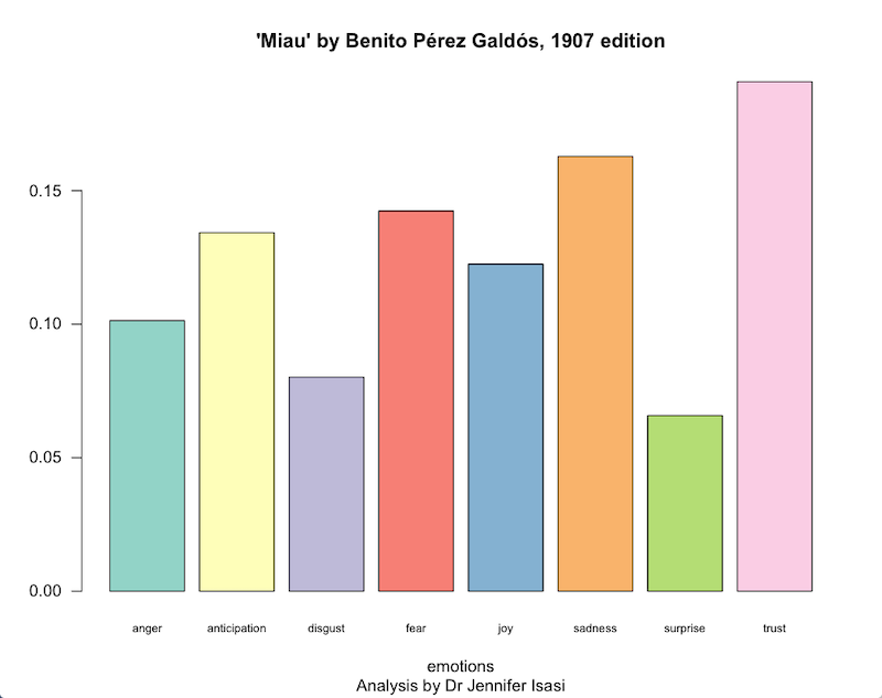
Figure 1: Bar chart showing the calculated scores of six emotions and two sub-emotions measured in the novel ‘Miau’ by Pérez Galdós.
If you are not interested in modifying these parameters, you could create a bar chart with default styling using the following code:
barplot(colSums(prop.table(sentiment_scores[, 1:8])))
Make sure you have enough space in the display window for the graph to draw properly, including space for the labels.
This information already indicates to us that the sadness and fear emotions are more prevalent than those of disgust or surprise. But what words does Galdós use to express fear? And how often does each emotionally charged word appear in the novel?
Counting Words by Emotion
One of the measures you can calculate using sentiment analysis is the frequency of words appearing in the text and how those words relate with each emotional category. To start with, you need to create a data object with all of the words that have a value greater than 0 – in this case you will start with those corresponding to the sadness column. In order to select only that column, use the dollar symbol $ after the name of your sentiment_scores variable to specify the name of the column you want to work with: sadness.
sad_words <- text_words[sentiment_scores$sadness> 0]
The contents of sad_words does not tell you much on its own, since it only offers you the list of relevant words without any further context. To also obtain the number of appearances of each ‘sadness’ word, you can generate a table. To get a quick look of some of the top entries, use the unlist and table functions along with the decreasing argument to display the matches in descending order (if you want ascending order, change TRUE to FALSE); you can create a new table object to print the first twelve words in the list, along with their frequency using the following code (see Table 2 for translations of the Spanish words):
sad_word_order <- sort(table(unlist(sad_words)), decreasing = TRUE)
head(sad_word_order, n = 12)

>            muy            nada           pobre           tarde
>            271             156              64              58
>            mal            caso            malo           salir
>             57              50              39              35
>          madre  insignificante              ay           culpa
>             33              29              24              22
Table 2: English translations of the Spanish words in the preceding code output block
| Spanish | English |
|---|---|
| muy | very |
| nada | nothing |
| pobre | poor |
| tarde | late |
| mal | bad |
| caso | case |
| malo | bad |
| salir | to leave |
| madre | mother |
| insignificante | insignificant |
| ay | ow! |
| culpa | fault |
If you want to know how many unique words are connected to sadness, you can use the length function on the newly created sad_word_order variable:
length(sad_word_order)

> [1] 349
You can repeat the same operation with the rest of the emotion categories, or those that you are interested in, as well as those with positive or negative sentiment scores. To make sure you understand how to adapt the code, try to obtain the results for the emotion ‘joy’ and compare them with ‘sadness’.9
Depending on the type of analysis that you want to conduct, this may be an efficient approach. For the purposes of this introductory lesson, you are also going next generate a word cloud to help visualise the terms associated with each emotional category (for demonstration purposes, you will use four).
An Emotional Word Cloud
In order to create a word cloud of terms that correspond with each emotion in Miau, you are going to first collect all words with an emotion score greater than 0. Similarly to the previous example, you use the $ symbol to specify which column of data (which emotion) you are interested in, indicating that you want entries with a value greater than 0.
If working on a machine running Windows, you will have to indicate to the programme if your text contains accented characters using the following approach:
On Mac and Linux
cloud_emotions_data <- c(
  paste(text_words[sentiment_scores$sadness> 0], collapse = " "),
  paste(text_words[sentiment_scores$joy > 0], collapse = " "),
  paste(text_words[sentiment_scores$anger > 0], collapse = " "),
  paste(text_words[sentiment_scores$fear > 0], collapse = " "))
On Windows
Windows needs an additional step to indicate the text is in UTF-8 format, which is done using the iconv function.
cloud_emotions_data <- c(
  paste(text_words[sentiment_scores$sadness> 0], collapse = " "),
  paste(text_words[sentiment_scores$joy > 0], collapse = " "),
  paste(text_words[sentiment_scores$anger > 0], collapse = " "),
  paste(text_words[sentiment_scores$fear > 0], collapse = " "))

cloud_emotions_data <- iconv(cloud_emotions_data, "latin1", "UTF-8")
Once you have collected the data for the four target emotions, you can organise it into four separate documents to use as the basis for creating each of your four word clouds:
cloud_corpus <- Corpus(VectorSource(cloud_emotions_data))
Next, you transform the corpus into a term-document matrix using the TermDocumentMatrix() function. Then you specify that you want the data organised as a matrix using the as.matrix() function.
To see the first few entries of this output, use the head function:
cloud_tdm <- TermDocumentMatrix(cloud_corpus)
cloud_tdm <- as.matrix(cloud_tdm)
head(cloud_tdm)

>               Docs
> Terms          1 2 3 4
>   abandonado   4 0 4 0
>   abandonar    1 0 0 0
>   abandonará   2 0 0 0
>   abandonaré   1 0 0 0
>   abandonarías 1 0 0 0
>   abandono     3 0 3 0
Now, rename the numbered columns with the relevant emotion words so that the output is more human-readable. Again, you can see the state of your dataset with the head function:
colnames(cloud_tdm) <- c('sadness', 'happiness', 'anger', 'joy')
head(cloud_tdm)

>               Docs
> Terms          sadness  happiness  anger     trust
>   abandonado          4         0      4         4
>   abandonar           1         0      0         1
>   abandonará          2         0      0         2
>   abandonaré          1         0      0         1
>   abandonarías        1         0      0         1
>   abandono            3         0      3         3
Finally, you can visualise these results as a word cloud. The font size of a word in a word cloud is linked to the frequency of its appearance in the document. We can also control a number of other aspects of the word cloud’s presentation.
To start, use the set.seed() function to ensure that while following along your outputs will look the same as in the example (if you don’t do this your output will have a randomised pattern and may not match the screenshots herein - which may not be important for your own research results but is helpful when following along).
To generate the cloud itself, use the comparison.cloud function from the R wordcloud package. In this example, you will indicate that the object cloud_tdm will have a non-random word order. You will also specify the colour scheme of each group of words, the title size, and general scale of the visualisation. To make the cloud readable, you will also specify a maximum number of terms. These parameters are all adjustable.
set.seed(757) # this can be set to any integer
comparison.cloud(cloud_tdm, random.order = FALSE,
                 colors = c("green", "red", "orange", "blue"),
                 title.size = 1, max.words = 50, scale = c(2.5, 1), rot.per = 0.4)
You should get an image similar to Figure 2 although with the location of the words altered since it is generated according to the size of the canvas.
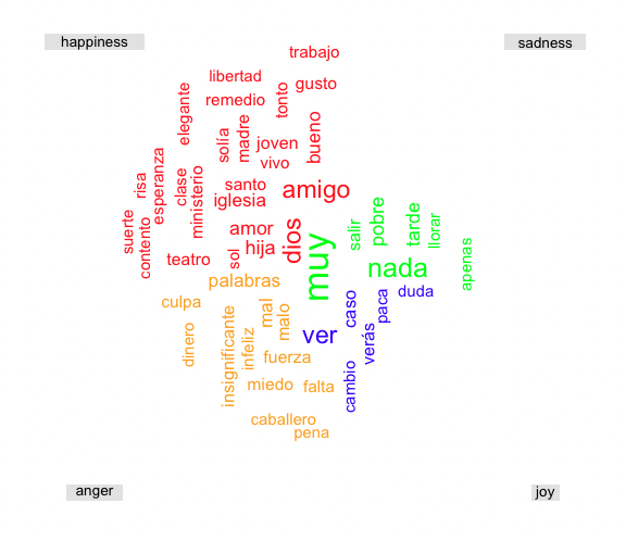
Figure 2: Word Cloud of most frequent words corresponding to sadness, happiness, anger, and joy in the novel ‘Miau’ by Pérez Galdós.
What does the word cloud suggest to you? Surely the connection of ‘very’ (muy) to the sadness emotion and of ‘money’ (dinero) to the anger emotion needs further consideration. These less obvious results are exactly what many scholars warn about when thinking about sentiment analysis, and demonstrate why a researcher must always ask if the outcomes of the analysis make sense before trying to draw any research conclusions from them. As noted, the sentiment analysis vocabulary used in this tutorial uses a vocabulary that’s been automatically translated from English, and is thus not perfect when used on Spanish-language text.
Visualising Emotion and Sentiment Across the Progression of a Text
To complement the isolated readings of emotions as above, you can also study the fluctuation of positive and negative sentiment across the text (Figure 3). R provides a way to both normalise and visualise this time-series sentiment analysis data. Since the sentiment analysis algorithm assigns both positive and negative sentiment scores, you need to generate data between a range of -1 (most negative moments) and 1 (most positive moments); 0 is considered neutral. To calculate these scores, you multiply the values in the negative values of the original sentiment_scores data table by -1 and then add the result to the positive values.
sentiment_valence <- (sentiment_scores$negative *-1) + sentiment_scores$positive
Finally, you can generate a graph with the simple_plot() function, which is built into the syuzhet package, and which offers you a choice of two different graphs; the first presents the various measurements calculated by the algorithm, and the second is a normalisation of those measures. The horizontal axis (X axis) presents the text in 100 normalised fragments and the vertical axis (Y axis) shows the strength of the sentiment in the text. Depending on the computing power of your machine, the graph may take 20 to 30 minutes to finish rendering.
simple_plot(sentiment_valence)
Make sure your graph display window is sized large enough to actually draw the graph. If it isn’t you will see the error message:
Error in plot.new() : figure margins too large.
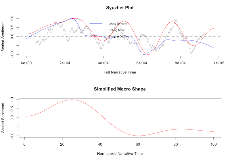
Figure 3: Evolution of the use of positive and negative sentiment through the novel ‘Miau’ by Pérez Galdós
Based on Figure 3, you might conclude that the novel Miau begins with fairly neutral language, transitions into moments of happiness early on, and moves into some quite negative description in the remaining pages, ending on a negative note, as indicated by the sample sentence we drew upon earlier in the lesson in which Villaamil dies. Anyone who has read the novel will know well the protagonist’s despair, so in this case the analysis matches a traditional reading of the text, which answers our research question about whether or not the automated sentiment analysis reflects a close reading of the text.
Save Your Data
If you want to save the data so that you can come back to it later, you can archive it in comma separates values (CSV) format, using the function write.csv(). This will save your main data table, sentiment_scores, which contains the results of the eight emotions and two sentiments we generated, and puts that into a CSV file. You can also add the keyword associated with each row in the left-most column to act as helpful labels.
write.csv(sentiment_scores, file = "analysis_sent_miau.csv", row.names = text_words)
Now you have all of the tools and knowledge you need to start to analyse your own texts and compare them with each other.
Loading your own Sentiment Lexicon
While the above introduction provides you with many tools for exploring sentiment analysis, this tutorial has not presented an exhaustive list of possibilities.
You may be working on a project in which you have already created a sentiment dictionary that you would like to use. Or perhaps you need to be able to customise a vocabulary and its corresponding sentiment scores to apply to a particular cultural or temporal context related to your research. Maybe you’re looking to improve upon the automatically translated results of the NRC lexicon used here. In each of those cases, as of mid 2022, you can also load your own lexicon dataset into the software using the custom function to repeat some of the calculations and visualisations used in this lesson.
To load your own sentiment lexicon, you first have to create or modify a dataframe containing at minimum a column of words and a column containing the corresponding scores for those words, which the author recommends saving in a CSV file format.
Try this example:
|word|value|
|---|---|
|amor|1|
|cólera|-1|
|alfombra|0|
|catástrofe|-2|
Next, to load your saved data from a CSV file, use the read.csv function, which will create a new dataset that you can access in R just as you have in the above examples (change ‘FILEPATH’ to the full location of your CSV file):
personalised_vocabulary <- read.csv("FILEPATH")
method <- "custom"
sentiments_sentences <- get_sentiment(sentences_vector, method = method, lexicon = personalised_vocabulary)
If you want to visualise sentiment across the progression of a text, you can use the plot function, which uses the same graphing parameters that you’ve already learned:
plot(sentiments_sentences,
   type = "l",
   main = "'Miau' by Benito Pérez Galdós, 1907 edition",
   sub = "Analysis by Dr Jennifer Isasi",
   xlab="emotions", ylab = " "
  )
Keep in mind that this form of customised analysis is limited, and that you may not be able to perform all of the same operations that we introduced above. For example, following the model example with your own dictionary, as you would not have information about emotions you would not be able to make a word cloud in the same way.
Works Cited
- Arnold, Taylor, and Lauren Tilton. ‘Basic Text Processing in R’, Programming Historian 6 (2017), https://doi.org/10.46430/phen0061
- Damasio, Antonio R. El error de Descartes: La razón de las emociones (Andres Bello, 1999).
- Dewar, Taryn. ‘R Basics with Tabular Data’, Programming Historian 5 (2016), https://doi.org/10.46430/phen0056.
- Gottschalk, Louis, and Goldine Gleser. The Measurement of Psychological States through the Content Analysis of Verbal Behaviour (University of California, 1969).
- Heuser, Ryan, Franco Moretti, Erik Steiner. ‘The Emotions of London’ Stanford Literary Lab, Pamphlet 13 (2016) 1-10.
- Hu, Minqing, and Bing Liu, ‘Mining and Summarizing Customer Reviews.’, Proceedings of the ACM SIGKDD International Conference on Knowledge Discovery & Data Mining (KDD-2004), 2004.
- Jockers, Matthew. ‘Introduction to the Syuzhet Package’ CRAN (2020), https://cran.r-project.org/web/packages/syuzhet/vignettes/syuzhet-vignette.html.
- Jockers, Matthew. ‘Some thoughts on Annie’s thoughts…about Syuzhet’ Matthew L. Jockers (2015), http://www.matthewjockers.net/page/2/.
- Leemans, Inger, Janneke M. van der Zwaan, Isa Maks, Erika Kujpers, Kristine Steenberge. ‘Mining Embodied Emotions: A Comparative Analysis of Sentiment and Emotion in Dutch Texts, 1600-1800’ Digital Humanities Quarterly 11 (2017).
- Liu, Bing. Sentiment Analysis and Opinion Mining (Morgan & Claypool, 2012).
- Meder, Theo, Dong Nguyen, Rilana Gravel. ‘The Apocalypse on Twitter’ Digital Scholarship in the Humanities 31 (2016), 398-410.
- Mohammad, Saif. ‘NRC Word-Emotion Association Lexicon’, National Research Council Canada (2010), https://saifmohammad.com/WebPages/NRC-Emotion-Lexicon.htm.
- Mohammad, Saif, and Peter D. Turney. ‘Crowdsourcing a Word–Emotion Association Lexicon’ Computational Intelligence 29 (2013): 436-465, doi: 10.1111/j.1467-8640.2012.00460.x.
- Nguyen, Thein Hai, Kiyoaki Shirai, Julien Velcin. ‘Sentiment Analysis on Social Media for Stock Movement Prediction’ Expert Systems with Applications 42 (2015), 9603-9611.
- Nielsen, Finn Årup. ‘AFINN Sentiment Lexicon’ (2009-2011).
- Pereira Zazo, Óscar. El analisis de la comunicación en español (Kendal Hunt, 2015).
- Pérez Galdós, Benito. Miau (La Guirnalda, 1888).
- Pérez Galdós, Benito. Miau (Sucesores de Hernando, 1907).
- Rodríguez Aldape, Fernando Manuel. Cuantificación del Interés de un usuario en un tema mediante minería de texto y análisis de sentimiento. (MA Thesis, Universidad Autónoma de Nuevo León, 2013).
- Schmidt, Thomas, Manuel Burghardt, Christian Wolff. ‘Towards Multimodal Sentiment Analysis of Historic Plays: A Case Study with Text and Audio for Lessing’s Emilia Galotti’ 4th Conference of the Association of Digital Humanities in the Nordic Countries (2019).
- Siddiqui, Nabeel. ‘Data Wrangling and Management in R’, Programming Historian 6 (2017), https://doi.org/10.46430/phen0063.
- Sprugnoli, Rachele, Sara Tonelli, Alessandro Marchetti, Giovanni Moretti. ‘Towards Sentiment Analysis for Historical Texts’ Digital Scholarship in the Humanities 31 (2016): 762-772.
- Stone, Philip, Dexter Dunphy, Marshall Smith. ‘The General Inquirer: A Computer Approach to Content Analysis’ (M.I.T. Press, 1966).
- Swafford, Annie. ‘Problems with the Syuzhet Package’ Anglophile in Academia (2015), https://annieswafford.wordpress.com/2015/03/02/syuzhet/.
- Wilkinson Saldaña, Zoë. ‘Sentiment Analysis for Exploratory Data Analysis,’ Programming Historian 7 (2018), https://doi.org/10.46430/phen0079
Notes
-
For example, see: Louis Gottschalk, Goldine Gleser (1969) The Measurement of Psychological States through the Content Analysis of Verbal Behaviour (University of California); Philip Stone, Dexter Dunphy, Marshall Smith (1966) ‘The General Inquirer: A Computer Approach to Content Analysis’ (M.I.T. Press); Bing Liu, (2012) Sentiment Analysis and Opinion Mining (Morgan & Claypool); Thein Hai Nguyen, Kiyoaki Shirai, Julien Velcin (2015). ‘Sentiment Analysis on Social Media for Stock Movement Prediction’ Expert Systems with Applications 42: 9603-9611; Theo Meder, Dong Nguyen, Rilana Gravel (2016). ‘The Apocalypse on Twitter’ Digital Scholarship in the Humanities 31 (2): 398-410. ↩
-
For some examples in English, see: Inger Leemans, Janneke M. van der Zwaan, Isa Maks, Erika Kujpers, Kristine Steenberge (2017). ‘Mining Embodied Emotions: A Comparative Analysis of Sentiment and Emotion in Dutch Texts, 1600-1800’ Digital Humanities Quarterly 11 (4); Rachele Sprugnoli, Sara Tonelli, Alessandro Marchetti, Giovanni Moretti (2016). ‘Towards Sentiment Analysis for Historical Texts’ Digital Scholarship in the Humanities 31 (4): 762-772; Thomas Schmidt, Manuel Burghardt, Christian Wolff (2019). ‘Towards Multimodal Sentiment Analysis of Historic Plays: A Case Study with Text and Audio for Lessing’s Emilia Galotti’ 4th Conference of the Association of Digital Humanities in the Nordic Countries; Ryan Heuser, Franco Moretti, Erik Steiner (2016). ‘The Emotions of London’ Stanford Literary Lab, Pamphlet 13: 1-10. ↩
-
Antonio R. Damasio, El Error de Descartes: La razón de las emociones. (Barcelona: Andres Bello, 1999). ↩
-
Óscar Pereira Zazo, El analisis de la comunicación en español (Iowa: Kendal Hunt, 2015), 32. ↩
-
‘Bing’: Minqing Hu and Bing Liu, ‘Mining and summarizing customer reviews.’, Proceedings of the ACM SIGKDD International Conference on Knowledge Discovery & Data Mining (KDD-2004), 2004; ‘Afinn’: Finn Årup Nielsen, ‘AFINN Sentiment Lexicon’ (2009-2011); ‘NRC’: Saif Mohammad, ‘NRC Word-Emotion Association Lexicon’, National Research Council Canada (2010). ↩
-
Saif Mohammad and Peter D. Turney, ‘Crowdsourcing a Word–Emotion Association Lexicon’, Computational intelligence 29 (2013): 436-465, doi: 10.1111/j.1467-8640.2012.00460.x ↩
-
Richard Socher, ‘Recursive Deep Learning for Natural Language Processing and Computer Vision’ PhD diss., (Stanford University, 2014). ↩
-
Thanks to Mounika Puligurthi, intern at the University of Texas (UT) Digital Scholarship Office (during the spring of 2019), for her help interpreting this calculation. ↩
-
There are more words assigned to the emotion sadness than to joy, both in total number of words (2,061 vs 1,552) and in unique words (349 vs 263). The word ‘Mother’ appears under both sadness and joy with a value of 33 points. What do you think the significance of that classification decision is? ↩