Contents
Introduction
A few years back, William Turkel wrote a series of blog posts called A Naive Bayesian in the Old Bailey, which showed how one could use machine learning to extract interesting documents out of a digital archive. This tutorial is a kind of an update on that blog essay, with roughly the same data but a slightly different version of the machine learner.
The idea is to show why machine learning methods are of interest to historians, as well as to present a step-by-step implementation of a supervised machine learner. This learner is then applied to the Old Bailey digital archive, which contains several centuries’ worth of transcripts of trials held at the Old Bailey in London. We will be using Python for the implementation.
One obvious use of machine learning for a historian is document selection. If we can get the computer to “learn” what kinds of documents we want to see, we can enlist its help in the always-time-consuming task of finding relevant documents in a digital archive (or any other digital collection of documents). We’ll still be the ones reading and interpreting the documents; the computer is just acting as a fetch dog of sorts, running to the archive, nosing through documents, and bringing us those that it thinks we’ll find interesting.
What we will do in this tutorial, then, is to apply a machine learner called Naive Bayesian to data from the Old Bailey digital archive. Our goals are to learn how a Naive Bayesian works and to evaluate how effectively it classifies documents into different categories - in this case, trials into offense categories (theft, assault, etc.). This will help us determine how useful a machine learner might be to us as historians: if it does well at this classification task, it might also do well at finding us documents that belong to a “class” we, given our particular research interests, want to see.
Step by step, we’ll do the following:
- learn what machine learners do, and look more closely at a popular learner called Naive Bayesian.
- download a set of trial records from the Old Bailey archive.
- write a script that saves the trials as text (removing the XML markup) and does a couple of other useful things.
- write a couple of helper scripts to assist in testing the learners.
- write a script that tests the performance of the learner.
Files you will need
save-trialtxts-by-category.pytenfold-crossvalidation.pycount-offense-instances.pypretestprocessing.pytest-nb-learner.pynaivebayes.pyenglish-stopwords.txt
A zip file of the scripts is available. You can also download another zip file containing the scripts, the data that we are using and the files that result from the scripts. (The second option is probably easiest if you want to follow along with the lesson, since it gives you everything you need in the correct folder structure.) More information about where to put the files is in the “Preliminaries” section of the part where we actually begin to code.
Note: You will not need any Python modules that don’t come with standard installations, except for BeautifulSoup (used in the data creation step, not in the learner code itself).
The Old Bailey Digital Archive
The Old Bailey digital archive contains 197,745 criminal trials held at the Old Bailey, aka the Central Criminal Court in London. The trials were held between 1674 and 1913, and since the archive provides the full transcript of each trial, many of which include testimony by defendants, victims, and witnesses, it’s a great resource for all kinds of historians interested in the lives of ordinary people in London.
What makes the collection particularly useful for our purposes is that the text of each trial is richly annotated with such information as what type of an offense was involved (pocketpicking, assault, robbery, conspiracy…), the name and gender of each witness, the verdict, etc. What’s more, this information has been added to the document in XML markup, which allows us to extract it easily and reliably. That, in turn, lets us train a machine learner to recognize the things we are interested in, and then test the learner’s performance.
Of course, in the case of the Old Bailey archive, we might not need this computer-assisted sorting all that badly, since the archive’s curators, making use of the XML markup, offer us a ready-made search interface that lets us look for documents by offense type, verdict, punishment, etc. But that’s exactly what makes the Old Bailey such a good resource for testing a machine learner: we can check how well the learner performs by checking its judgments against the human-annotated information in the Old Bailey documents. That, in turn, helps us decide how (or whether) a learner could help us explore other digital document collections, most of which are not as richly annotated.
Machine learning
Machine learning can mean a lot of different things, but the most common tasks are classification and clustering.
Classification is performed by supervised learners — “supervised” meaning that a human assistant helps them learn, and only then sends them out to classify by themselves. The basic training procedure is to give the learner labeled data: that is, we give it a stack of things (documents, for example) where each of those things is labeled as belonging to a group. This is called training data. The learner then looks at each item in the training data, looks at its label, and learns what distinguishes the groups from each other. To see how well the learner learned, we then test it by giving it data that is similar to the training data but that the learner hasn’t seen before and that is not labeled. This is called (you guessed it!) test data. How well the learner performs on classifying this previously-unseen data is a measure of how well it has learned.
The classic case of a supervised classifier is a program that separates junk email (spam) from regular email (ham). Such a program is “trained” by giving it a lot of spam and ham to look at, along with the information of which is which. It then builds a statistical model of what a spam message looks like versus what a regular email message looks like. So it learns that a message is more likely to be spam if it contains sexual terms, or words like “offer” and “deal”, or, as things turn out, “ff0000,” the HTML code for red. It can then apply that statistical model to incoming messages and discard the ones it identifies as spam.
Clustering is usually a task for unsupervised learners. An unsupervised learner doesn’t get any tips on how the data “ought” to be sorted, but rather is expected to discover patterns in the data automatically, grouping the data by the patterns it has discovered. Unlike in supervised classification, in unsupervised clustering we don’t tell the learner what the “right” groups are, or give it any hints on what items in the data set should go together. Rather, we give it data with a bunch of features, and (often, but not always) we tell it how many groups we want it to create. The features could be anything: in document clustering, they are normally words. But clustering isn’t limited to grouping documents: it could also be used in, say, trying to improve diagnoses by clustering patient records. In that task, the features would be various attributes of the patient (age, weight, blood pressure, presence and quality of various symptoms etc.) and the clustering algorithm would attempt to create groups that share as many features as closely as possible.
A side note: Some of you may have come to think of an objection to this supervised/unsupervised distinction: namely, that the clustering method is not entirely “unsupervised” either. After all, we tell it what features it should look at, whether it is words (rather than sentences, or two-word sequences, or something else) in a document, or a list of numeric values in a patient record. The learner never encounters the data entirely unprepared. Quite true. But no matter - the distinction between unsupervised and supervised is useful nevertheless, in that in one we tell the learner what the right answer is, and in the other it comes to us with some pattern it has figured out without an answer key. Each is useful for different kind of tasks, or sometimes for different approaches to the same task.
In this tutorial, we are dealing with a supervised learner that we train to perform document classification. We give our learner a set of documents along with their correct classes, and then test it on a set of documents they haven’t seen, with the hope that it will succeed in guessing the document’s correct classification.
A Naive Bayesian learner
A Naive Bayesian is a supervised learner: we give it things marked with group labels, and its job is basically to learn the probability that a thing that looks a particular way belongs in a particular group.
But why “naive”? And what “Bayesian”?
“Naive” simply means that the learner makes the assumption that all the “features” that make up a document are independent of each other. In our case, the features are words, and so the learner assumes that the occurrence of a particular word is completely independent of the occurrence of another word. This, of course, is often not true, which is why we call it “naive.” For example, when we put “new” and “york” together to form “New York,” the result has a very different meaning than the “new” and “york” in “New clothes for the Prince of York.” If we were to distinguish “New York” from “New” and “York” occurring separately, we might find that each tends to occur in very different types of documents, and thus not identifying the expression “New York” might throw our classifier off course.
Despite their simplistic assumption that the occurrence of any particular feature is independent of the occurrence of other features, Naive Bayesian classifiers do a good enough job to be very useful in many contexts (much of the real-world junk mail detection is performed by Naive Bayesian classifiers, for example). Meanwhile, the assumption of independence means that processing documents is much less computationally intensive, so a Naive Bayesian classifier can handle far more documents in a much shorter time than many other, more complex methods. That in itself is useful. For example, it wouldn’t take too long retrain a Naive Bayesian learner if we accumulated more data. Or we could give it a bigger set of data to begin with; a pile of data that a Naive Bayesian could burrow through in a day might take a more complex method weeks or even months to process. Especially when it comes to classification, more data is often as significant as a better method — as Bob Mercer of IBM famously quipped in 1985, “there is no data like more data.”
As for the “Bayesian” part, that refers to the 18th-century English minister, statistician, and philosopher Thomas Bayes. When you google for “Naive Bayesian,” you will turn up a lot of references to “Bayes’ theorem” or “Bayes’ rule,” which is a formula for applying conditional probabilities (the probability of some thing X, given some other thing Y).
Bayes’ theorem is related to Naive Bayesian classifiers, in that we can formulate the classification question as “what is the probability of document X, given class Y?” However, unless you’ve done enough math and probability to be comfortable with that kind of thinking, it may not provide the easiest avenue to grasping how a Naive Bayesian classifier works. Instead, let’s look at the classifier in a more procedural manner. (Meanwhile, if you prefer, you can check out an explanation of Bayes’ rule and conditional probabilities that does a very nice job and is also a good read.)
Understanding Naive Bayesian classification using a generative story
To understand Naive Bayesian classification, we will start by telling a story about how documents come into being. Telling such a story — called a “generative story” in the business — often simplifies the probabilistic analysis and helps us understand the assumptions we’re making. Telling the story takes a while, so bear with me. There is a payoff at the end: the story directly informs us how to build a classifier under the assumptions that the particular generative story makes.
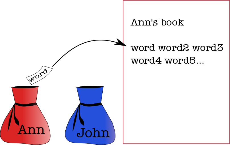
The fundamental assumption we will make in our generative story is that documents come into being not as a result of intellectual cogitation but as a result of a process whereby words are picked at random out of a bag and then put into a document (known as a bag-of-words model).
So we pretend that historical works, for example, are written in something like the following manner. Each historian has his or her own bag of words with a vocabulary specific to that bag. So when Ann the Historian writes a book, what she does is this:
- She goes to the bag that is her store of words.
- She puts her hand in and pulls out a piece of paper.
- She reads the word on the piece of paper, writes it down in her book, and puts the paper back in the bag.
- Then she again puts her hand in the bag and pulls out a piece of paper.
- She writes down that word in the book, and puts the piece of paper back in the bag.
Ann the Historian keeps going until she decides her book (or article, or blog post, or whatever) is finished. The next time she wants to write something, she goes back to her bag of words and does the same thing. If her friend John the Historian were to write a book, he would go to his own bag, which has a different set of words, and then he would follow the same procedure of taking out a word, writing it down, putting it back in. It’s just one damn word after another.
Bags of Words
(If this procedure sounds familiar, that may be because it sounds a bit like the generative story told in explaining how topic modeling works. However, the story in topic modeling is a bit different in that, for instance, each document contains words from more than one class. Also, you should note that topic modeling is unsupervised — you don’t tell the modeler what the “right” topics are, it comes up with them all by itself.)
So let’s say you are a curator of a library of historical works, and one day you discover a huge forgotten trunk in the basement of the library. It turns out that the trunk contains dozens and dozens of typed book manuscripts. After some digging, you find a document that explains that these are transcripts of unpublished book drafts by three historians: Edward Gibbon, Carl Becker, and Mercy Otis Warren.
What a find! But unfortunately, as you begin sorting through the drafts, you realize that they are not marked with the author’s name. What can you do? How can you classify them correctly?
Well, you do have other writings by these authors. And if historians write their documents in the manner described above — if each historian has his or her own bag of words with a particular vocabulary and a particular distribution of words — then we can figure out who wrote each document by looking at the words it contains and comparing the distribution of those words to the distribution of words in documents we know were written by Gibbon, Becker, and Warren, respectively.
So you go to your library stacks and get out all the books by Gibbon, Becker, and Warren. Then you start counting. You start with Edward Gibbon’s oeuvre. For each word in a work by Gibbon, you add the word to a list marked “Gibbon.” If the word is already in the list, you add to its count. Then you do the same with the works of Mercy Otis Warren and Carl Becker. Finally, for each author, you add up the total number of words you’ve seen. You also add up the total number of monographs you have examined so you’ll have a metric for how much work each author has published.
So what you end up with is something like this:
| Edward Gibbon (5) | Carl Becker (18) | Mercy Otis Warren (2) |
|---|---|---|
| empire, 985 | everyman, 756 | revolution, 989 |
| rome, 897 | revolution, 699 | constitution, 920 |
| fall, 887 | philosopher, 613 | principles, 899 |
| … | … | … |
| (total), 352,003 | (total), 745,532 | (total), 300,487 |
What you have done, in essence, is to reconstruct each historian’s “bag of words” — now you know (at least approximately) what words each historian uses and in what proportions. Armed with this representation of the word distributions in the works of Gibbons, Becker, and Warren, you’re ready to tackle the task of figuring out who wrote which manuscripts.
You’re going to work manuscript by manuscript and author by author, first pretending that the manuscript you’re currently considering was written by Gibbons, then that it was written by Becker, and so on. For each author, you calculate how likely it is that the manuscript really was written by that author.
So with your first manuscript in hand, you start by assuming that the manuscript was written by Gibbons. First you figure out the overall probability of any monograph being written by Gibbons rather than either of the two others — that is, of the Gibbons bag rather than the Becker bag or the Warren bag being used to produce a monograph. You do this by taking the number of books written by Gibbons and dividing it by the total number of books written by all these authors. That comes out to 5/25, or 0.2 (20 percent).
Then, you start looking at the words in the manuscript. Let’s say the first word is “fall.” You check how often that word occurred in Gibbons’ published oeuvre, and you find that the answer is 887. Then you check how many words, overall, there were in Gibbons’ total works, and you note that the answer is 352,003. You divide 887 by 352,003 to get the proportional frequency (call it p) of “fall” in Gibbons’ work (0.0025). For the next word, you do the same procedure, and then multiply the probabilities together (you multiply since each action — picking an author, or picking a word — represents an independent choice). In the end you end with a tally like this:
p_bag * p_word_1 * p_word_2 * ... * p_word_n
Note that including the probability of picking the bag (p_bag) is an important step: if you only go by the words in the manuscript and ignore how many manuscripts (or rather, published works) each author has written, you can easily go wrong. If Becker has written ten times the number of books that Warren has, it should reasonably require much firmer evidence in the form of an ample presence of “Warrenesque” words to assume that a manuscript was written by Warren than that it was written by Becker. “Extraordinary claims require extraordinary evidence,” as Carl Sagan once said.
OK, so now you have a total probability of the manuscript having been written by Gibbons. Next, you repeat the whole procedure with the assumption that maybe it was instead written by Becker (that is, that it came out of the bag of words that Becker used when writing). That done, you move on to considering the probability that the author was Warren (and if you had more authors, you’d keep going until you had covered each of them).
When you’re done, you have three total probabilities — one probability per author. Then you just pick out the largest one, and, as they say, Bob’s your uncle! That’s the author who most probably wrote this manuscript.
(Minor technical note: when calculating
p_bag * p_word1 * ... * p_word_n
in a software implementation we actually work with the logarithms of the probabilities since the numbers easily become very small. When doing this, we actually calculate
log(p_bag) + log(p_word1) + ... + log(p_word_n)
That is, our multiplications turn into additions in line with the rules of logarithms. But it all works out right: the class with the highest number at the end wins.)
But wait! What if a manuscript contains a word that we’ve never seen Gibbons use before, but also lots of words he used all the time? Won’t that throw off our calculations?
Indeed. We shouldn’t let outliers throw us off the scent. So we do something very “Bayesian”: we put a “prior” on each word and each class — we pretend we’ve seen all imaginable words at least (say) once in each bag, and that each bag has produced at least (say) one document. Then we add those fake pretend counts — called priors, or pseudocounts — to our real counts. Now, no word or bag gets a count of zero.
In fact, we can play around with the priors as much as we like: they’re simply a way of modeling our “prior belief” in the probability of one thing over another. They could model our assumptions about a particular author being more likely than others, or a particular word being more likely to have come from the bag of a specific author, and so on. Such beliefs are “prior” in the sense that we hold the belief before we’ve seen the evidence we are considering in the actual calculation we are making. So above, for example, we could add a little bit to Mercy Otis Warren’s p_bag number if we thought it likely that as a woman, she might well have had a harder time getting published, and so there might reasonably be more manuscript material from her than one might infer from a count of her published monographs.
In some cases, priors can make a Naive Bayesian classifier much more usable. Often when we’re classifying, after all, we’re not after some abstract “truth” — rather, we simply want a useful categorization. In some cases, it’s much more desirable to be mistaken one way than another, and we can model that with proper class priors. The classic example is, again, sorting email into junk mail and regular mail piles. Obviously, you really don’t want legitimate messages to be deleted as spam; that could do much more damage than letting a few junk messages slip through. So you set a big prior on the “legitimate” class that causes your classifier to only throw out a message as junk when faced with some hefty evidence. By the same token, if you’re sorting the results of a medical test into “positive” and “negative” piles, you may want to weight the positive more heavily: you can always do a second test, but if you send the patient home telling them they’re healthy when they’re not, that might not turn out so well.
So there you have it, step by step. You have applied a Naive Bayesian to the unattributed manuscripts, and you now have three neat piles. Of course, you should keep in mind that Naive Bayesian classifiers are not perfect, so you may want to do some further research before entering the newfound materials into the library catalog as works by Gibbons, Becker, and Warren, respectively.
OK, so let’s code already!
So, our aim is to apply a Naive Bayesian learner to data from the Old Bailey. First we get the data; then we clean it up and write some routines to extract information from it; then we write the code that trains and tests the learner.
Before we get into the nitty-gritty of downloading the files and examining the training/testing script, let’s just summarize what our aim is and what the basic procedure looks like.
We want to have our Naive Bayesian read in trial records from the Old Bailey and do with them the same thing as we did above in the examples about the works of Gibbons, Becker, and Warren. In that example, we used the published works of these authors to reconstruct each historian’s bag of words, and then used that knowledge to decide which historian had written which unattributed manuscripts. In classifying the Old Bailey trials, we will give the learner a set of trials labeled with the offense for which the defendant was indicted so it can figure out the “bag of words” that is associated with that offense. Then the learner will use that knowledge to classify another set of trials where we have not given it any information about the offense involved. The goal is to see how well the learner can do this: how often does it label an unmarked trial with the right offense?
The procedure used in the scripts we employ to train the learner is no more complicated than the one in the historians-and-manuscripts example. Basically, each trial is represented as a list of words, like so:
michael, carney, was, indicted, for, stealing, on, the, 22nd, of, december, 26lb, weight, of, nails, value, 7s, 18, dozen, of, screws, ...
... , the, prisoners, came, to, my, shop, on, the, night, in, question, and, brought, in, some, ragged, pieces, of, beef, ...
..., i, had, left, my, door, open, and, when, i, returned, i, missed, all, this, property, i, found, it, at, the, pawnbroker, ...
When we train the learner, we give it a series of such word lists, along with their correct bag labels (correct offenses). The learner then creates word lists for each bag (offense), so that it ends up with a set of counts similar to the counts we created for Gibbons, Becker, and Warren, one count for each offense type (theft, deception, etc.)
When we test the learner, we feed it the same sort of word lists representing other trials. But this time we don’t give it the information about what offense was involved. Instead, the learner does what we did above: when it gets a list of words, it compares that list to the word counts for each offense type, calculating which offense type has a bag of words most similar to this list of words. It works offense by offense, just like we worked author by author. So first it assumes that the trial involved, say, the offense “theft”. It looks at the first word in the trial’s word list, checks how often that word occurred in the “theft” bag, performs its probability calculations, moves on to the next word, and so on. Then it checks the trial’s word list against the next category, and the next, until it has gone through each offense. Finally it tallies up the probabilities and labels the trial with the offense category that has the highest probability.
Finally, the testing script evaluates the performance of the learner and lets us know how good it was at guessing the offense associated with each trial.
Preliminaries
Many of the tools we are using to deal with the preliminaries have been discussed at Programming Historian before. You may find it helpful to check out (or revisit) the following tutorials:
- Milligan & Baker, Introduction to the Bash Command Line
- Milligan, Automated Downloading with wget
- Knox, Understanding Regular Expressions
- Wieringa, Intro to Beautiful Soup
A few words about the file structure the scripts assume/create:
I have a “top-level” directory, which I’m calling bailey (you could call it something else, it’s not referenced in the code). Under that I have two directories: baileycode and baileyfiles. The first contains all the scripts; the second contains the files that are either downloaded or created by the scripts. That in turn has subdirectories; all except one (for the downloaded XML files — see below) are created by the scripts.
If you downloaded the complete zip package with all the files and scripts, you automatically get the right structure; just unpack it in its own directory. The only files that are omitted from that are the zip files of trials downloaded below (if you got the complete package, you already have the unpacked contents of those files, and the zips would just take up unnecessary space).
If you only downloaded the scripts, you should do the following:
- Create a directory and name it something sensible (say, bailey).
- In that directory, create another directory called baileycode and unpack the contents of the script zip file into that directory (make sure you don’t end up with two baileycode directories inside one another).
- In the same directory (bailey), create another directory called baileyfiles.
On my Mac, the structure looks like this:
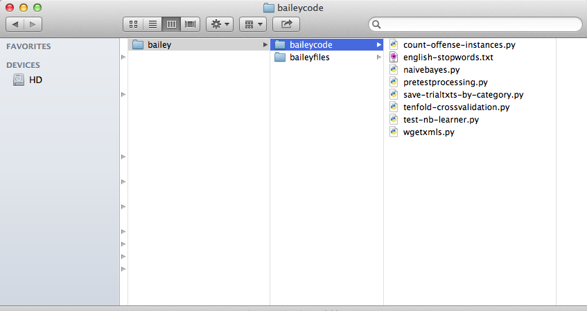
Bailey Folders
Downloading trials
The Old Bailey lets you download trials in zip files of 10 trials each, so that’s what we’ll do. This is how we do it: we first look at how the Old Bailey system requests files, and then we write a script that creates a file with a bunch of those requests. Then we feed that file to wget, so we don’t have to sit by our computers all day downloading each set of 10 trials that we want.
As explained on the Old Bailey documentation for developers page, this is what the http request for a set of trials looks like:
http://www.oldbaileyonline.org/obapi/ob?term0=fromdate_18300114&term1=todate_18391216&count=10&start=211&return=zip
As you see, we can request all trials that took place between two specified dates (fromdate and todate). The count specifies how many trials we want, and the start variable says where in the results to start (in the above, we start with result number 211 and get the ten following trials). Ten seems to be the highest number allowed for count, so we need to work around that.
We get around the restriction for how many trials can be in a zip file with a little script that builds as many of the above type of requests as we need to get all trials from the 1830s. We can find out how many trials that is by going to the Old Bailey search page and entering January 1830 as the start date, December 1839 as the end date, and choosing “Old Bailey Proceedings > trial accounts” in the “Search In” field. Turns out there were 22,711 trials in the 1830s.
Here’s the whole script (wgetxmls.py) that creates the list of http requests we need:
    mainoutdirname = '../baileyfiles/'
    wgets = ''
    for x in range(0,22711,10):
        getline = 'http://www.oldbaileyonline.org/obapi/ob?term0=fromdate_18300114&term1=todate_18391216&count=10&start=' + str(x+1) + '&return=zip\n'
        wgets += getline
    filename = mainoutdirname + 'wget1830s.txt'
    with open(filename,'w') as f:
        f.write(wgets)
As you see, we accept the limitation of 10 trials at a time, but manipulate the start point until we have covered all the trials from the 1830s.
Assuming you’re in the baileycode directory, you can run the script from the command line like this:
python wgetxmls.py
What that gets us is a file that looks like this:
http://www.oldbaileyonline.org/obapi/ob?term0=fromdate_18300114&term1=todate_18391216&count=10&start=1&return=zip
http://www.oldbaileyonline.org/obapi/ob?term0=fromdate_18300114&term1=todate_18391216&count=10&start=11&return=zip
http://www.oldbaileyonline.org/obapi/ob?term0=fromdate_18300114&term1=todate_18391216&count=10&start=21&return=zip
...
This file is saved in the baileyfiles directory; it is called wget1830s.txt.
To download the trials, create a new directory under baileyfiles; call it trialzips. Then go into that directory and call wget with the file we just created. So, assuming you are still in the baileycode directory, you would write the following commands on the command line:
cd ../baileyfiles
mkdir trialzips
cd trialzips
wget -w 2 -i ../wget1830s.txt
The “-w 2” is just to be polite and not overload the server; it tells
wget to wait 2 seconds between each request. The “-i” flag tells wget
that it should request the URLs found in wget1830s.txt.
What wget returns is a lot of zip files that have unwieldy names and no
extension. You should rename these so that the extension is “.zip”.
Then, in the directory baileyfiles, create a subdirectory called
1830s-trialxmls and then unpack the zips into that so that it
contains 22,170 XML files that each look like t18391216-388.xml. Assuming
you are still in the trialzips directory, you would write:
for f in * ; do mv $f $f.zip; done;
mkdir ../1830s-trialxmls
unzip "*.zip" -d ../1830s-trialxmls/
If you open one of the trial XMLs in a browser, you can see that it contains all kinds of useful information: name and gender of defendant, name and gender of witnesses, type of offense, and so on. Here’s a snippet from one trial:
<persname id="t18300114-2-defend110" type="defendantName">
THOMAS TAYLOR
    <interp inst="t18300114-2-defend110" type="surname" value="TAYLOR">
    <interp inst="t18300114-2-defend110" type="given" value="THOMAS">
    <interp inst="t18300114-2-defend110" type="gender" value="male">
    <interp inst="t18300114-2-defend110" type="age" value="25">
</interp></interp></interp></interp></persname>
was indicted for
    <rs id="t18300114-2-off7" type="offenceDescription">
        <interp inst="t18300114-2-off7" type="offenceCategory" value="violentTheft">
        <interp inst="t18300114-2-off7" type="offenceSubcategory" value="robbery">
            feloniously assaulting
        <persname id="t18300114-2-victim112" type="victimName">
            David Grant
                  <interp inst="t18300114-2-victim112" type="surname" value="Grant">
            <interp inst="t18300114-2-victim112" type="given" value="David">
            <interp inst="t18300114-2-victim112" type="gender" value="male">
            <join result="offenceVictim" targorder="Y" targets="t18300114-2-off7 t18300114-2-victim112">
        </join></interp></interp></interp></persname>
</interp></interp></rs>
The structured information in the XML lets us reliably extract the “classes” we want to sort our documents into. We are going to classify the trials by offense category (and subcategory), so that’s the information we’re going to extract before converting the XML into a text file that we can then feed to our learner.
Saving the trials into text files
Now that we have the XML files, we can start extracting information and plain text from them to feed to our learner. We want to sort the trials into text files, so that each text file contains all the trials in a particular offense category (theft-simplelarceny, breakingpeace-riot, etc.).
We also want to create a text file that contains all the trial IDs (marked in the XML), so we can use that to easily create cross-validation samples. The reasons for doing this are discussed below in the section “Creating the cross-validation samples”.
The script that does these things is called save-txttrials-by-category.py
and it’s pretty extensively commented, so I’ll just note a few things here.
- We strip the trial text of all punctuation, including quote marks and parentheses, and we equalize all spaces (newlines, tabs, multiple spaces) into a single space. This helps us simplify the coding of the training process (and, incidentally, keep the code that trains the learner general enough that as long as you have text files saved in the same format as we use here, you should be able to apply it more or less directly to your data).
- That of course makes the text hard to read for a human. Therefore, we also save the text of each trial into a file named after the trial id, so that we can easily examine a particular trial if we want to (which we will).
The script creates the following directories and files under baileyfiles:
- Directory 1830s-trialtxts: this will contain the text file versions of the trials after they have been stripped of all XML formatting. Each file is named after the trial’s ID.
- Directory 1830s-trialsbycategory: this
will contain the text files that represent all the text in all the
trials belonging to a particular category. These are named after the
category, e.g.,
theft-simplelarceny.txt. Each category file contains all the trials in that category, with one trial per line. - File
trialids.txt. This contains the sorted list of trial IDs, one ID per line; we will use it later in creating cross-validation samples for training the learner (this is the next step). - Files
offensedict.jsonandtrialdict.json. These json files will come into use in training the learner.
So if you’re still in the trialxmls directory, you would write the following commands to run this script:
cd ../../baileycode/
python save-trialtxts-by-category.py
This will take a while. After it’s done, you should have the directories and files described above.
Creating the cross-validation samples
Now that we have all our trials saved where we want them, all we need to do is to create the cross-validation samples and we’re ready to test our learners.
Cross-validation simply means repeatedly splitting our data into chunks, some of which we use for training and others for testing. Since the idea is to get a learner to extract information from one set of documents that it can then use to determine the class of documents it has never seen, we obviously have to reserve a set of documents that are unknown to the learner if we want to test its performance. Otherwise it’s a bit like letting your students first read an exam and its answers and then have them take that same exam. That would only tell you how closely they read the actual exam, not whether they’ve learned something more general.
So what you want to do is to test the learner on data it hasn’t seen before, so that you can tell whether it has learned some general principles from the training data. You could just split your data into two sets, using, say, 80 percent for training and 20 percent for testing. But a common practice is to split your data repeatedly into different test and train sets, so that you can ensure that your test results aren’t the consequence of some oddball quirk in the portion of data you left for testing.
Two scripts are involved in creating the cross-validation sets. The
script tenfold-crossvalidation.py creates
the samples. It reads in the list of trial ids we created in the
previous step, shuffles that list to make it random, and divides it into
10 chunks of roughly equal length (that is, a roughly equal number of
trial ids). Then it writes those 10 chunks each into its own text file,
so we can read them into our learner code later. Next, to be meticulous,
we can run the count-offense-instances.py
to confirm that if we are interested in a particular trial category,
that category is reasonably evenly distributed across the samples.
Before you run the count-offense-instances.py script, you should
edit it to set the category to the one you’re interested in and let the
script know whether we’re looking at a broad or a specific category.
This is what the relevant part of the code looks like:
indirname = '../baileyfiles/'
offensedict_fn = indirname + 'offensedict.json'
offensecat = 'breakingpeace' #change to target category
broadcat = True #set true if category is e.g. "theft" instead of "theft-simplelarceny"
And here are the commands to run the cross-validation scripts (assuming you are still in the baileycode directory).
python tenfold-crossvalidation.py
python count-offense-instances.py
Alternatively, you can run them using pypy, which is quite a bit faster.
pypy tenfold-crossvalidation.py
pypy count-offense-instances.py
The output of the count-offense-instances.py script looks like
this:
Offense category checked for: breakingpeace
sample0.txt: 31
sample1.txt: 25
sample2.txt: 32
sample3.txt: 25
sample4.txt: 36
sample5.txt: 33
sample6.txt: 29
sample7.txt: 35
sample8.txt: 27
sample9.txt: 31
From the output, we can conclude that the distribution of instances of
“breakingpeace” is more or less even. If it isn’t, we can re-run the
tenfold-crossvalidation.py script, and then check the distribution again.
Testing the learner
All right, we are ready to train and test our Naive Bayesian! The script
that does this is called test-nb-learner.py. It starts by defining a few
variables:
categoriesdir = '../baileyfiles/1830s-trialsbycategory/'
sampledirname = '../baileyfiles/Samples_1830s/' #location of 10-fold cross-validation
stopwordfilename = '../baileyfiles/english-stopwords.txt'
# the ones below should be set to None if not using
cattocheck = 'breakingpeace' #if evaluating recognition one category against rest
pattern = '[^-]+' #regex pattern to use if category is not complete filename
Most of these are pretty self-explanatory, but note the two last ones. The variable “cattocheck” determines whether we are looking to identify a specific category or to sort each trial into its proper category (the latter is done if the variable is set to None). The variable “pattern” tells us whether we are using the whole file name as the category designation, or only a part of it, and if the latter, how to identify the part. In the example above, we are focusing on the broad category “breakingpeace”, and so we are not using the whole file name, which would be e.g. “breakingpeace-riot” but only the part before the dash. Before you run the code, you should set these variables to what you want them to be.
Note that “cattocheck” here should match the “offensecat” that you
checked for with the count-offense-instances.py script. No error is
produced if it does not match, and it’s fairly unlikely that it will
have any real impact, but if the categories don’t match, then of course
you have no assurance that the category you’re actually interested in is
more or less evenly distributed across the ten cross-validation samples.
Note also that you can of course set “cattocheck” to “None” and leave the pattern as it is, in which case you will be sorting into the broader categories.
So, with the basic switches set and knobs turned, we begin by reading in
all the trials that we have saved. We do this with the function called
process_data that can be found in the pretestprocessing.py file. (That file
contains functions that are called from the scripts you will run, so it
isn’t something you’ll run directly at any point.)
print 'Reading in the data...'
trialdata = ptp.process_data(categoriesdir,stopwordfilename,cattocheck,pattern)
The process_data function reads in all the files in the directory that contains our trial category files, and processes them so that we get a list containing all the categories and the trials belonging to them, with the trial text lowercased and tokenized (split into a list of words), minus stopwords (common words like a, the, me, which, etc.) Each trial begins with its id number, so that’s one of our words (though we ignore it in training and testing). Like this:
    [
     [breakingpeace,
       ['trialid','victim','peace','disturbed','man','tree',...]
       ['trialid','dress','blood','head','incited',...]
      ...]
     [theft,
       ['trialid','apples','orchard','basket','screamed','guilty',....]
       ['trialid','rotten','fish']
      ...]
    ]
Next, making use of the results of the ten-fold cross-validation routine
we created, we loop through the files that define the
samples, each time making one sample the test set and the rest the train
set. Then we split ‘trialdata’, the list of trials-by-category that we
just created, into train and test sets accordingly. The functions that
do these two steps are create_sets and
splittraintest, both in the pretestprocessing.py file.
Now we train our Naive Bayesian classifier on the train set. The classifier we are using (which is included in the scripts zip file) is one written by Mans Hulden, and it does pretty much exactly what the “identify the author of the manuscript” example above describes.
    # split train and test
    print 'Creating train and test sets, run {0}'.format(run)
    trainsetids, testsetids = ptp.create_sets(sampledirname,run)
    traindata, testdata = ptp.splittraintest(trainsetids,testsetids,trialdata)

    # train learner
    print 'Training learner, run {0}...'.format(run)
    mynb = nb.naivebayes()
    mynb.train(traindata)
After the learner is trained, we are ready to test how well the it performs. Here’s the code:
    print 'Testing learner, run {0}...'.format(run)

    for trialset in testdata:
        correctclass = trialset[0]
        for trial in trialset[1:]:
            result = mynb.classify(trial)
            guessedclass =  max(result, key=result.get)
            # then record correctness of classification result
            # note that first version does a more complex evaluation
            # ... for two-way (one class against rest) classification
            if cattocheck:
                if correctclass == cattocheck:
                    catinsample += 1
                if guessedclass == cattocheck:
                     guesses += 1
                     if guessedclass == correctclass:
                         hits += 1
            if guessedclass == correctclass:
                correctguesses += 1

            total +=1
So we loop through the categories in the “testdata” list (which is of the same format as the “trialdata” list). For each category, we loop through the trials in that category, classifying each trial with our Naive Bayesian classifier, and comparing the result to the correct class (saved in the first element of each category list within the testdata list.) Then we add to various counts to be able to evaluate the results of the whole classification exercise.
To run the code that trains and tests the learner, first make sure you have edited it to set the “cattocheck” and “pattern” switches, and then call it on the command line (assuming you’re still in the directory baileycode):
python test-nb-learner.py
Again, for greater speed, you can also use pypy:
pypy test-nb-learner.py
The code will print out some accuracy measures for the classification task you have chosen. The output should look something like this:
Reading in the data...
Creating train and test sets, run 0
Training learner, run 0...
Testing learner, run 0...
Creating train and test sets, run 1
Training learner, run 1...
...
Training learner, run 9...
Testing learner, run 9...
Saving correctly classified trials and close matches...
Calculating accuracy of classification...
Two-way classification, target category breakingpeace.
And the results are:
Accuracy 99.00%
Precision: 61.59%
Recall: 66.45%
Average number of target category trials in test sample per run: 30.4
Average number of trials in test sample per run: 2271.0
Obtained in 162.74 seconds
Next, let’s take a look at what these measures of accuracy mean.
Measures of classification
The basic measure of classification prowess is accuracy: how often did classifier guess the class of a document correctly? This is calculated by simply dividing the number of correct guesses by the total number of documents considered.
If we’re interested in a specific category, we can extract a bit more data. So if we set, for example, cattocheck = ‘breakingpeace’, like above, we can then examine how well the classifier did with respect to the “breakingpeace” category in particular.
So, in the testlearner code, if we’re doing multiway classification, we only record how many trials we’ve seen (“total”) and how many of our guesses were correct (“correctguesses”). But if we’re considering a single category, say “breakingpeace,” we record a few more numbers. First, we keep track of how many trials belonging to the category “breakingpeace” there are in our test sample (this tally is in “catinsample”). We also keep track of how many times we’ve guessed that a trial belongs to the “breakingpeace” category (“guesses”). And finally we record how many times we have guessed correctly that a trial belongs to “breakingpeace” (“hits”).
Now that we have this information, we can use it to calculate a couple of standard measures of classification efficiency: precision and recall. Precision tells us how often we correctly guessed that a trial was in the “breakingpeace” category. Recall lets us know what proportion of the “breakingpeace” trials we caught.
Let’s take another example to clarify precision and recall. Imagine you want all the books on a particular topic — World War I, say — from your university library. You send out one of your many minions (all historians possess droves of them, as you know) to get the books. The minion dutifully returns with a big pile.
Now, suppose you were in possession of a list that contained of every single book in the library on WWI and no books that weren’t related to the WWI. You could then check the precision and recall of your minion with regard to the category of “books on WWI.”
Recall is the term for the proportion of books on WWI in the library that your minion managed to grab. That is, the more books on WWI remaining in the library after your minion’s visit, the lower your minion’s recall.
Precision, in turn, is the term for the proportion of books in the pile brought by your minion that actually had to do with WWI. The more irrelevant (off-topic) books in the pile, the lower the precision.
So, say the library has 1,000 books on WWI, and your minion lugs you a pile containing 400 books, of which 300 have nothing to do with WWI. The minion’s recall would be (400-300)/1,000, or 10 percent. The minion’s precision, in turn, would be (400-300)/400, or 25 percent.
(Should have gone yourself, eh?)
A side note: the minion’s overall accuracy — correct guesses divided by actual number of examples — would be:
(the number of books on WWI in your pile - the number of books *not* on
WWI in your pile + the number of books in the library *not* on WWI)
------------------------------------------------------------------------
the total number of books in the library
So if the library held 100,000 volumes, this would be (100 - 300 + 99,000) / 100,000 — or 98.8 percent. That seems like a great number, but since it merely means that your minion was smart enough to leave most of the library books in the library, it’s not very helpful in this case (except inasmuch as it is nice not to be buried under 100,000 volumes.)
How well does our Naive Bayesian do?
Our tests on the Naive Bayesian use the data set consisting of all the trials from the 1830s. It contains 17,549 different trials in 50 different offense categories (which can be grouped into 9 broad categories).
If we run the Naive Bayesian so that it attempts to sort all trials into their correct broad categories, its accuracy is pretty good: 94.3 percent. So 94 percent of the time, when it considers how it should sort trials in the test sample into “breakingpeace,” “deception,” “theft,” and so on, it chooses correctly.
For the more specific categories (“theft-simplelarceny,” “breakingpeace-riot,” and so on) the same exercise is much less accurate: then, the classifier gets it right only 72 percent of the time. That’s no wonder, really, given that some of the categories are so small that we barely have any examples. We might do a bit better with more data (say, all the trials from the whole 19th century, instead of only all the trials from the 1830s).
The first, overall category results are pretty impressive. They give us quite a bit of confidence that if what we needed to do was to sort documents into piles that weren’t all too fine-grained, and we had a nice bunch of training data, a Naive Bayesian could do the job for us.
But the problem for a historian is often rather different. A historian using a Naive Bayesian learner is more likely to want to separate documents that are “interesting” from documents that are “not interesting” — usually meaning documents dealing with a particular issue or not dealing with it. So the question is really more one where we have a mass of “uncategorized” or “other” documents and a much smaller set of “interesting” documents, and we try to find more of the latter among the former.
In our current exercise, that situation is fairly well represented by trying to identify documents from a single category in the mass of the rest of the documents, set to category “other.” So how well are we able to do that? In other words, if we set cattocheck = ‘breakingpeace’ (or another category) so that all trials get marked as either that category or as “other,” and then run the classifier, what kinds of results do we get?
Well, our overall accuracy is still high: over 95 percent in all cases for the broad categories, and usually about that for the detailed ones as well. But just like the minion going off to the library to get books on WWI had a pretty high accuracy because he/she didn’t bring back half the library, in this case, too, our accuracy is mostly just due to the fact that we manage to not misidentify too many “other” trials as being in the category we’re interested in. Because there are so many “other” trials, those correct assessments far outweigh the minus points we may have gotten from missing interesting trials.
Precision and recall, therefore, are more in this case more interesting measures than overall accuracy. Here’s a table showing precision and recall for each of the “broad” categories in our trial sample, and for a few sample detailed categories. The last column shows how many target category trials there were in the test set on average (remember, we did ten runs with different train/test splits, so all our results are averages of that).
Naive Bayesian classifier, two-way classification, 10-fold cross-validation
Broad categories
| Category | Precision (%) | Recall (%) | Avg # trials in cat in TeS |
|---|---|---|---|
| breakingpeace | 63.52 | 64.05 | 24.2 |
| damage | 0.00 | 0.00 | 1.2 |
| deception | 53.47 | 61.43 | 47.7 |
| kill | 62.5 | 89.39 | 17.9 |
| miscellaneous | 47.83 | 4.44 | 24.8 |
| royaloffenses | 85.56 | 91.02 | 42.3 |
| sexual | 93.65 | 49.17 | 24.0 |
| theft | 96.26 | 98.75 | 1551.8 |
| violenttheft | 68.32 | 33.01 | 20.9 |
Sample detailed categories
| Category | Precision (%) | Recall (%) | Avg # trials in cat in TeS |
|---|---|---|---|
| theft-simplelarceny | 64.37 | 89.03 | 805.9 |
| theft-receiving | 92.21 | 61.53 | 198.1 |
| deception-forgery | 74.29 | 11.87 | 21.9 |
| violenttheft-robbery | 68.42 | 31.86 | 20.4 |
| theft-extortion | 0.00 | 0.00 | 1.3 |
There are a few generalizations we can make from these numbers.
First, it’s obvious that if the category is too small, we are out of luck. So for “damage,” a small enough broad category that our test samples only held a little over one instance of it on average, we get no results. Similarly, in the detailed categories, when the occurrence of cases per test sample drops into the single digits, we fail miserably. This is no wonder: if the test sample contains about one case on average, there can’t be much more than ten cases total in the whole data set. That’s not much to go on.
Second, size isn’t everything. Although we do best for the biggest category, theft (which in fact accounts for over half our sample), there are some smaller categories we do very well for. We have very high recall and precision for “royaloffenses,” a mid-sized category, and very high recall plus decent precision for “kill,” our smallest reasonable-sized category. A reasonable guess would be that the language that occurs in the trials is distinctive and, in the case of “royaloffenses,” doesn’t occur much anywhere else. Meanwhile, unsurprisingly, we get low scores for the “miscellaneous” category. We also have high precision for the “sexual” category, indicating that it has some language that doesn’t tend to appear anywhere else — though we miss about half the instances of it, which would lead us to suspect that many of the trials in that category omit some of the language that most distinguishes it from others.
Third, in this sample at least, there seems to be no clear pattern regarding whether the learner has better recall or better precision. Sometimes it casts a wide net that drags in both a good portion of the category and some driftwood, and sometimes it handpicks the trials for good precision but misses a lot that don’t look right enough for its taste. So in half the cases here, our learner has better precision than recall, and in half better recall than precision. The differences between precision and recall are, however, bigger for the cases where precision is better than recall. That isn’t necessarily a good thing for us, since as historians we might be happier to see more of the “interesting” documents and do the additional culling ourselves than to have our learner miss a lot of good documents. We’ll return to the question of the meaning of classification errors below.
Extracting the most indicative features
The naivebayes.py script has a feature
that allows you to extract the most (and least) indicative features of
your classification exercise. This allows you to see what weighs a lot
in the learner’s mind — what it has, in effect, learned.
The command to issue is: mynb.topn_print(10) (for the 10 most indicative; you can put in any number you like). Here are the results for a multi-way classification of the broad categories in our data:
deception ['norrington', 'election', 'flaum', 'polish', 'caton', 'spicer', 'saltzmaun', 'newcastle', 'stamps', 'rotherham']
royaloffences ['mould', 'coster', 'coin', 'caleb', 'counterfeit', 'obverse', 'mint', 'moulds', 'plaster-of-paris', 'metal']
violenttheft ['turfrey', 'stannard', 'millward', 'falcon', 'crawfurd', 'weatherly', 'keith', 'farr', 'ventom', 'shurety']
damage ['cow-house', 'ewins', 'filtering-room', 'fisk', 'calf', 'skirting', 'girder', 'clipping', 'saturated', 'firemen']
breakingpeace ['calthorpe-street', 'grievous', 'disable', 'mellish', 'flag', 'bodily', 'banner', 'aforethought', 'fursey', 'emerson']
miscellaneous ['trevett', 'teuten', 'reitterhoffer', 'quantock', 'feaks', 'boone', 'bray', 'downshire', 'fagnoit', 'ely']
kill ['vault', 'external', 'appearances', 'slaying', 'deceased', 'marchell', 'disease', 'pedley', 'healthy', 'killing']
theft ['sheep', 'embezzlement', 'stealing', 'table-cloth', 'fowls', 'dwelling-house', 'missed', 'pairs', 'breaking', 'blankets']
sexual ['bigamy', 'marriage', 'violate', 'ravish', 'marriages', 'busher', 'register', 'spinster', 'bachelor', 'married']
Some of these make sense instantly. In “breakingpeace” (which includes assaults, riots and woundings) you can see the makings of phrases like “grievous bodily harm” and “malice aforethought,” along with other indications of wreaking havoc like “disable” and “harm.” In royaloffenses, the presence of “mint,” “mould” and “plaster-of-paris” make sense since the largest subcategory is coining offenses. In “theft,” one might infer that sheep, fowl, and table-cloths seem to have been popular objects for stealing (though table-cloth may of course have been a wrapping for stolen objects; one would have to examine the trials to know).
Others are more puzzling. Why is violenttheft almost exclusively composed of what seem to be person or place names? Why is “election” indicative of deception? Is there a lot of election fraud going on, or abuse of elected office? Looking at the documents, one finds that 9 of the words indicative of violent theft are person names, and one is a pub; why person and pub names should be more indicative here than for other categories is mildly intriguing and might bear further analysis (or might just be a quirk of our data set — remember that “violenttheft” is a fairly small category). As for “election,” it’s hard to distinguish a clear pattern, though it seems to be linked to fraud attempts on and by various officials at different levels of government.
The indicative features, then, may be intriguing in themselves (though obviously, one should not draw any conclusions about them without closely examining the data first). They are also useful in that they can help us determine whether something is skewing our results in a way we don’t wish, something we may be able to correct for with different weighting or different selection of features (see the section on Tuning below).
The meanings of misclassification
Again, it’s good to keep in mind that in classifying documents we are not always after an abstract “true” classification, but simply a useful or interesting one. Thus, it is a good idea to look a bit more closely at the “errors” in classification.
We’ll focus on two-way classification, and look at the cases where the Naive Bayesian incorrectly includes a trial in a category (false positives) as well as take a look at trials it narrowly excludes from the category (let’s call them close relatives).
In the script for testing the learner (test-nb-learner.py), we saved the trial ids for
false positives and close relatives so we could examine them later.
Here’s the relevant code bit:
result = mynb.classify(trial)
guessedclass =  max(result, key=result.get)
if cattocheck:
    diff = abs(result[cattocheck] - result['other'])
    if diff < 10 and guessedclass != cattocheck:
        closetrials.append(trial[0])
        difflist.append(diff)
    if correctclass == cattocheck:
        catinsample += 1
    if guessedclass == cattocheck:
         guesses += 1
         if guessedclass == correctclass:
             hits += 1
         else:
             falsepositives.append(trial[0])
if guessedclass == correctclass:
    correctguesses += 1
False positives are easy to catch: we simply save the cases where we guessed that a trial belonged to the category but it really did not.
For close relatives, we first check how confident we were that the trial did not belong in our category. When we issue the call to classify the trial mynb.classify(trial), it returns us a dictionary that looks like this:
{
    'other': -2358.522248351527,
    'violenttheft-robbery': -2326.2878233211086
}
So to find the close relatives, we compare these two values, and if the difference between them is small, we save the id of the trial we are currently classifying into a list of close relatives. (In the code chunk above, we have rather arbitrarily defined a “small” difference as being under 10).
At the end of the script, we write the results of these operations into
two text files: falsepositives.txt and closerelatives.txt.
Let’s look more closely at misclassifications for the category “violenttheft-robbery.” Here are the first 10 rows of the close relatives file and the first 20 rows of the false positives file, sorted by offense:
Close relatives
breakingpeace-wounding, t18350105-458, 1.899530878
theft-pocketpicking, t18310407-90, 0.282424548
theft-pocketpicking, t18380514-1168, 0.784184742
theft-pocketpicking, t18301028-208, 0.797341405
theft-pocketpicking, t18341016-85, 1.296811989
violenttheft-robbery, t18370102-317, 1.075548985
violenttheft-robbery, t18350921-2011, 1.105672712
violenttheft-robbery, t18310407-204, 1.521788666
violenttheft-robbery, t18370102-425, 1.840718222
violenttheft-robbery, t18330214-13, 2.150018805
False positives
breakingpeace-assault, t18391021-2933
breakingpeace-wounding, t18350615-1577
breakingpeace-wounding, t18331017-159
breakingpeace-wounding, t18350615-1578
breakingpeace-wounding, t18330704-5
kill-manslaughter, t18350706-1682
kill-manslaughter, t18360919-2161
kill-manslaughter, t18380618-1461
kill-murder, t18330103-7
kill-murder, t18391021-2937
miscellaneous-pervertingjustice, t18340904-144
theft-pocketpicking, t18300114-128
theft-pocketpicking, t18310407-66
theft-pocketpicking, t18330905-92
theft-pocketpicking, t18370703-1639
theft-pocketpicking, t18301028-127
theft-pocketpicking, t18310106-87
theft-pocketpicking, t18331017-109
theft-pocketpicking, t18320216-108
theft-pocketpicking, t18331128-116
The first thing we notice is that many of the close relatives are in fact from our target category — they are cases that our classifier has narrowly missed. So saving these separately could compensate nicely for an otherwise low recall number.
The second thing we notice is that more of the false positives seem to have to do with violence, whereas more of the close relatives seem to have to do with stealing; it seems our classifier has pegged the violence aspect of robberies as more significant in distinguishing them than the filching aspect.
The third thing we notice is that theft-pocketpicking is a very common category among both the close relatives and the false positives. And indeed, if we look at a sample trial from violenttheft-robbery and another from among the close pocketpicking relatives, we notice that there are definitely close similarities.
For example, trial t18310407-90, the closest close relative, involved a certain Eliza Williams indicted for pocketpicking. Williams was accused of stealing a watch and some other items from a certain Thomas Turk; according to Turk and his friend, they had been pub-crawling, Eliza Williams (whom they did not know from before) had tagged along with them, and at one point in the evening had pocketed Turk’s watch (Turk, by this time, was quite tipsy). Williams was found guilty and sentenced to be confined for one year.
Meanwhile, in trial t18300708-14, correctly classed as violenttheft-robbery, a man called Edward Overton was accused of feloniously assaulting a fellow by the name of John Quinlan. Quinlan explained that he had been out with friends, and when he parted from them he realized it was too late to get into the hotel where he worked as a waiter and (apparently) also had lodgings. Having nowhere to go, he decided to visit a few more public-houses. Along the way, he met Overton, whom he did not know from before, and treated him to a few drinks. But then, according to Quinlan, Overton attacked him as they were walking from one pub to another, and stole his watch as well as other possessions of his. According to Overton, however, Quinlan had given him the watch as a guarantee that he would repay Overton if Overton paid for his lodging for the night. Both men, it seems, were thoroughly drunk by the end of the evening. Overton was found not guilty.
Both trials, then, are stories of groups out drinking and losing their possessions; what made the latter a trial for robbery rather than for pocketpicking was simply Quinlan’s accusation that Overton had “struck him down.” For a historian interested in either robberies or pocketpickings (or pub-crawling in 1830s London), both would probably be equally interesting.
In fact, the misclassification patterns of the learner indicate that even when data is richly annotated, such as in the case of the Old Bailey, using a machine learner to extract documents may be useful for a historian: in this case, it would help you extract trials from different offense categories that share features of interest to you, regardless of the offense label.
Tuning
The possibilities for tuning are practically endless.
For example, you might consider tweaking your data. For instance, instead of giving your classifier all the words in the document, you might present it with a reduced set.
One way of reducing the number of words is to collapse different words together through stemming. So the verb forms “killed,” “kills,” “killing” would all become “kill” (as would the plural noun “kills”). A popular stemmer is the Snowball Stemmer, and you could add that to the tokenization step. (I ran a couple of tests with this, and while it made the process much slower, it didn’t much improve the results. But that would probably depend a bit on the kind of data you have.)
Another way is to select the words you give to the classifier according to some principle. One common solution is to pick only the words with a high TF-IDF score. TF-IDF is short for “term frequency - inverse document frequency,” and a high score means that the term occurs quite frequently in the document under consideration but rarely in documents in general. (You can also check out a more detailed explanation of TF-IDF, along with some Python code for calculating it.)
Other options include simply playing with the size of the priors: now, the Naive Bayesian has a class prior as well as a feature prior of 0.5, meaning that it pretends to have seen all classes and all words at least one-half times. Doing test runs with different priors might get you different results.
In addition to simply changing the general prior sizes, you might
consider having the classifier set a higher prior on the target
category than on the “other” category, in effect requiring less
evidence to include a trial in the target category. It might be worth
a try particularly since we noted above when examining the close
relatives (under Meanings of Misclassification) that many of them were
in fact members of our target category. Setting a larger prior on the
target class would probably catch those cases, boosting the recall. At
the same time, it probably would also lower the precision. (To change
the priors, you need to edit the naivebayes.py script.)
As you can see, there is quite a lot of fuzziness here: how you pick the features, how you pick the priors, and how you weight various priors all affect the results you get, and how to pick and weight is not governed by hard logic but is rather a process of trial and error. Still, like we noted noted in the section on the meaning of classification error above, if your goal is to get some interesting data to do historical analysis on, some fuzziness may not be such a big problem.
Happy hunting!