
Contents
- Introduction
- The Federalist Papers - Historical Context
- Our Test Cases
- Preparing the Data for Analysis
- First Stylometric Test: Mendenhall’s Characteristic Curves of Composition
- Second Stylometric Test: Kilgariff’s Chi-Squared Method
- Third Stylometric Test: John Burrows’ Delta Method (Advanced)
- Further Reading and Resources
- Acknowledgements
- Endnotes
Introduction
Stylometry is the quantitative study of literary style through computational distant reading methods. It is based on the observation that authors tend to write in relatively consistent, recognizable and unique ways. For example:
- Each person has their own unique vocabulary, sometimes rich, sometimes limited. Although a larger vocabulary is usually associated with literary quality, this is not always the case. Ernest Hemingway is famous for using a surprisingly small number of different words in his writing,1 which did not prevent him from winning the Nobel Prize for Literature in 1954.
- Some people write in short sentences, while others prefer long blocks of text consisting of many clauses.
- No two people use semicolons, em-dashes, and other forms of punctuation in the exact same way.
The ways in which writers use small function words, such as articles, prepositions and conjunctions, has proven particularly telling. In a survey of historical and current stylometric methods, Efstathios Stamatatos points out that function words are “used in a largely unconscious manner by the authors, and they are topic-independent.”2 For stylometric analysis, this is very advantageous, as such an unconscious pattern is likely to vary less, over an author’s corpus, than his or her general vocabulary. (It is also very hard for a would-be forger to copy.) Function words have also been identified as important markers of literary genre and of chronology.
Scholars have used stylometry as a tool to study a variety of cultural questions. For example, a considerable amount of research has studied the differences between the ways in which men and women write3 or are written about.4 Other scholars have studied the ways in which a sudden change in writing style within a single text may indicate plagiarism,5 and even the manner in which lyrics penned by musicians John Lennon and Paul McCartney grew progressively less cheerful and less active as the Beatles approached the end of their recording career in the 1960s.6
However, one of the most common applications of stylometry is in authorship attribution. Given an anonymous text, it is sometimes possible to guess who wrote it by measuring certain features, like the average number of words per sentence or the propensity of the author to use “while” instead of “whilst”, and comparing the measurements with other texts written by the suspected author. This is what we will be doing in this lesson, using as our test case perhaps the most famous instance of disputed authorship in political writing history, that of the Federalist Papers.
Learning Outcomes
At the end of this lesson, we will have examined the following topics:
- How to apply several stylometric methods to infer authorship of an anonymous text or set of texts.
- How to use relatively advanced data structures, including dictionaries of strings and dictionaries of dictionaries, in Python.
- The basics of the Natural Languate Toolkit (NLTK), a popular Python module dedicated to natural language processing.
Prior Reading
If you do not have experience with the Python programming language or are finding examples in this tutorial difficult, the author recommends you read the lessons on Working with Text Files in Python and Manipulating Strings in Python. Please note, that those lessons were written in Python version 2 whereas this one uses Python version 3. The differences in syntax between the two versions of the language can be subtle. If you are confused at any time, follow the examples as written in this lesson and use the other lessons as background material. (More precisely, the code in this tutorial was written using Python 3.6.4; the f-string construct in the line with open(f'data/federalist_{filename}.txt', 'r') as f:, for example, requires Python 3.6 or a more recent version of the language.)
Required materials
This tutorial uses both datasets and software that you will have to download and install.
The Dataset
To work through this lesson, you will need to download and unzip the archive of the Federalist Papers (.zip) containing the 85 documents that we will use for our analysis. The archive also contains the original Project Gutenberg ebook version of the Federalist Papers from which these 85 documents have been extracted. When you unzip the archive, it will create a directory called data in your current working directory. Make sure that you stay in this current working directory and that you save all work here while completing the lesson.
The Software
This lesson uses the following Python language versions and libraries:
- Python 3.x - the latest stable version is recommended.
- nltk - Natural Language Toolkit, usually abbreviated
nltk. - matplotlib
Some of these modules may not be pre-installed on your computer. Should you encounter error messages such as: “Module not found” or similar, you will have to download and install the missing module(s). This is easiest to accomplish using the pip command. Full details are available via the Programming Historian lesson on Installing Python modules with pip.
Some Notes about Language Independence
This tutorial applies stylometric analysis to a set of English-language texts using a Python library called nltk. Much of the functionality provided by the nltk works with other languages. As long as a language provides a clear way to distinguish word boundaries within a word, nltk should perform well. Languages such as Chinese for which there is no clear distinction between word boundaries may be problematic. I have used nltk with French texts without any trouble; other languages that use diacritics, such as Spanish and German, should also work well with nltk. Please refer to nltk’s documentation for details.
Only one of the tasks in this tutorial requires language-dependent code. To divide a text into a set of French or Spanish words, you will need to specify the appropriate language as a parameter to nltk’s tokenizer, which uses English as the default. This will be explained in the tutorial.
Finally, note that some linguistic tasks, such as part-of-speech tagging, may not be supported by nltk in languages other than English. This tutorial does not cover part-of-speech tagging. Should you need it for your own projects, please refer to the nltk documentation for advice.
The Federalist Papers - Historical Context
The Federalist Papers (also known simply as the Federalist) are a collection of 85 seminal political theory articles published between October 1787 and May 1788. These papers, written as the debate over the ratification of the Constitution of the United States was raging, presented the case for the system of government that the U.S. ultimately adopted and under which it lives to this day. As such, the Federalist is sometimes described as America’s greatest and most lasting contribution to the field of political philosophy.
Three of the Early Republic’s most prominent men wrote the papers:
- Alexander Hamilton, first Secretary of the Treasury of the United States.
- James Madison, fourth President of the United States and the man sometimes called the “Father of the Constitution” for his key role at the 1787 Constitutional Convention.
- John Jay, first Chief Justice of the United States, second governor of the State of New York, and diplomat.
However, who wrote which of the papers was a matter of open debate for 150 years, and the co-authors’ behavior is to blame for the mystery.
First, the Federalist was published anonymously under the shared pseudonym “Publius”. Anonymous publication was not uncommon in the eighteenth century, especially in the case of politically sensitive material. However, in the Federalist’s case, the fact that three people shared a single pseudonym makes it difficult to determine who wrote which part of the text. Compounding the problem is the fact that the three authors wrote about closely related topics, at the same time, and using the same cultural and political references, which made their respective vocabularies hard to distinguish from each other.
Second, because Madison and Hamilton left conflicting testimonies regarding their roles in the project. In a famous 1944 article, historian Douglass Adair7 explained that neither man wanted the true authorship of the Papers to become public knowledge during their lifetimes, because they had come to regret some of what they had written. The notoriously vainglorious Hamilton, however, wanted to make sure that posterity would remember him as the driving force behind the Papers. In 1804, two days before he was to fight a duel (in which he was killed), Hamilton wrote a note claiming 63 of the 85 Papers as his own work and gave it to a friend for safekeeping. Ten years later, Madison refuted some of Hamilton’s claims, stating that he was the author of 12 of the papers on Hamilton’s list and that he had done most of the work on three more for which Hamilton claimed equal credit. Since Hamilton was long dead, it was impossible for him to respond to Madison.
Third, because in the words of David Holmes and Richard Forsyth,8 Madison and Hamilton had “unusually similar” writing styles. Frederick Mosteller and Frederick Williams calculated that, in the papers for which authorship is not in doubt, the average lengths of the sentences written by the two men are both uncommonly high and virtually identical: 34.59 and 34.55 words respectively.9 The standard deviations in the lengths of the two men’s sentences are also nearly identical. And as Mosteller quipped, neither man was known to use a short word when a long one would do. Thus, there was no easy way to pinpoint any given paper as clearly marked with Hamilton’s or Madison’s stylistic signature.
It wasn’t until 1964 that Mosteller and David Lee Wallace10, using word usage statistics, came up with a relatively satisfactory solution to the mystery. By comparing how often Madison and Hamilton used common words like may, also, an, his, etc., they concluded that the disputed papers had all been written by Madison. Even in the case of Federalist 55, the paper for which they said that the evidece was the least convincing, Mosteller and Wallace estimated the odds that Madison was the author at 100 to 1.
Since then, the authorship of the Federalist has remained a common test case for machine learning algorithms in the English-speaking world.11 Stylometric analysis has also continued to use the Federalist to refine its methods, for example as a test case while looking for signs of hidden collaborations between multiple authors in a single text.12 Interestingly, some of the results of this research suggest that the answer to the Federalist mystery may not be quite as clear-cut as Mosteller and Wallace thought, and that Hamilton and Madison may have co-written more of the Federalist than we ever suspected.
Our Test Cases
In this lesson, we will use the Federalist as a case study to demonstrate three different stylometric approaches.
- Mendenhall’s Characteristic Curves of Composition
- Kilgariff’s Chi-Squared Method
- John Burrows’ Delta Method
This will require splitting the papers into six categories:
- The 51 papers known to have been written by Alexander Hamilton.
- The 14 papers known to have been written by James Madison.
- Four of the five papers known to have been written by John Jay.
- Three papers that were probably co-written by Madison and Hamilton and for which Madison claimed principal authorship.
- The 12 papers disputed between Hamilton and Madison.
- Federalist 64 in a category of its own.
This division mostly follows Mosteller’s lead13. The one exception is Federalist 64, which everyone agrees was written by John Jay but which we keep in a separate category for reasons that will become clear later.
Our first two tests, using T. C. Mendenhall’s characteristic curves of composition and Adam Kilgariff’s chi-squared distance, will look at the 12 disputed papers as a group, to see whether they resemble anyone’s writing in particular. Then, in our third and final test, we will apply John Burrows’ Delta method to look at Federalist 64 and to confirm whether it was, indeed, written by John Jay.
Preparing the Data for Analysis
Before we can proceed with stylometric analysis, we need to load the files containing all 85 papers into convenient data structures in computer memory.
The first step in this process is to assign each of the 85 papers to the proper set. Since we have given each paper standardized names from federalist_1.txt to federalist_85.txt, it is possible to assign each paper to its author (or to its test set, if we want to learn its author’s identity) using a Python dictionary. The dictionary is a data type made up of an arbitrary number of key-value pairs; in this case, the names of authors will serve as keys, while the lists of paper numbers will be the values associated with these keys.
papers = {
    'Madison': [10, 14, 37, 38, 39, 40, 41, 42, 43, 44, 45, 46, 47, 48],
    'Hamilton': [1, 6, 7, 8, 9, 11, 12, 13, 15, 16, 17, 21, 22, 23, 24,
                 25, 26, 27, 28, 29, 30, 31, 32, 33, 34, 35, 36, 59, 60,
                 61, 65, 66, 67, 68, 69, 70, 71, 72, 73, 74, 75, 76, 77,
                 78, 79, 80, 81, 82, 83, 84, 85],
    'Jay': [2, 3, 4, 5],
    'Shared': [18, 19, 20],
    'Disputed': [49, 50, 51, 52, 53, 54, 55, 56, 57, 58, 62, 63],
    'TestCase': [64]
}
Python dictionaries are very flexible. For example, we can access a value by indexing the dictionary with one of its keys, we can scan the entire dictionary by looping over its list of keys, etc. We will make ample use of this functionality as we move along.
Next, as we are interested in each author’s vocabulary, we will define a short Python function that creates a long listing of the words in each of the papers assigned to a single author. This will be stored as a string. Open your chosen Python development environment. If you do not know how to do this, you should read Setting up an Integrated Development Environment (Mac), (Linux), (Windows) before continuing.
# A function that compiles all of the text files associated with a single author into a single string
def read_files_into_string(filenames):
    strings = []
    for filename in filenames:
        with open(f'data/federalist_{filename}.txt', 'r') as f:
            strings.append(f.read())
    return '\n'.join(strings)
Third, we build a new data structure by repeatedly calling the read_files_into_string() function, passing it a different list of papers every time. We will store the results into another dictionary, this one with author/test case names as keys and all of the text of the relevant papers as values. For simplicity’s sake, we will refer to the string containing a list of papers as “the author’s corpus”, even when we are dealing with disputed or shared papers rather than with an individual’s known contribution.
# Make a dictionary out of the authors' corpora
federalist_by_author = {}
for author, files in papers.items():
    federalist_by_author[author] = read_files_into_string(files)
To make sure that the files loaded properly, print the first hundred characters of each dictionary entry to screen:
for author in papers:
    print(federalist_by_author[author][:100])
If this printing operation yields anything at all, then the file input operation has worked as expected and you can move on to stylometric analysis.
First Stylometric Test: Mendenhall’s Characteristic Curves of Composition
Literary scholar T. C. Mendenhall once wrote that an author’s stylistic signature could be found by counting how often he or she used words of different lengths.14 For example, if we counted word lengths in several 1,000-word or 5,000 word segments of any novel, and then plotted a graph of the word length distributions, the curves would look pretty much the same no matter what parts of the novel we had picked. Indeed, Mendenhall thought that if one counted enough words selected from various parts of a writer’s entire life’s work (say, 100,000 or so), the author’s “characteristic curve” of word length usage would become so precise that it would be constant over his or her lifetime.
By today’s standards, counting word lengths seems like a very blunt way of measuring literary style. Mendenhall’s method does not take the actual words in an author’s vocabulary into account, which is obviously problematic. Therefore, we should not treat the characteristic curves as a particularly trustworthy source of stylometric evidence. However, Mendenhall published his theory over one hundred and thirty years ago and made all calculations by hand. It is understandable that he would have chosen to work with a statistic that, however coarse, was at least easy to compile. In honor of the historical value of his early attempt at stylometry, and because the characteristic curve yields interesting visual results that can be implemented quickly, we will use Mendenhall’s method as a first step in our exploration of authorship attribution techniques.
The code required to calculate characteristic curves for the Federalist’s authors is as follows:
# Load nltk
import nltk
nltk.download('punkt')
%matplotlib inline

# Compare the disputed papers to those written by everyone,
# including the shared ones.
authors = ("Hamilton", "Madison", "Disputed", "Jay", "Shared")

# Transform the authors' corpora into lists of word tokens
federalist_by_author_tokens = {}
federalist_by_author_length_distributions = {}
for author in authors:
    tokens = nltk.word_tokenize(federalist_by_author[author])

    # Filter out punctuation
    federalist_by_author_tokens[author] = ([token for token in tokens
                                            if any(c.isalpha() for c in token)])

# Get a distribution of token lengths
token_lengths = [len(token) for token in federalist_by_author_tokens[author]]
federalist_by_author_length_distributions[author] = nltk.FreqDist(token_lengths)
federalist_by_author_length_distributions[author].plot(15,title=author)
The ‘%matplotlib inline’ declaration below ‘import nltk’ is required if your development environment is a Jupyter Notebook, as it was for me while writing this tutorial; otherwise you may not see the graphs on your screen. If you work in Jupyter Lab, please replace this clause with ‘%matplotlib ipympl’.
The first line in the code snippet above loads the Natural Language Toolkit module (nltk), which contains an enormous number of useful functions and resources for text processing. We will barely touch its basics in this lesson; if you decide to explore text analysis in Python further, I strongly recommend that you start with nltk’s documentation.
The next few lines set up data structures that will be filled by the block of code within the for loop. This loop makes the same calculations for all of our “authors”:
- It invokes
nltk’sword_tokenize()method to chop an author’s corpus into its component tokens, i.e., words, numbers, punctuation, etc.; - It looks at this list of tokens and filters out non-words;
- It creates a list containing the lengths of every word token that remains;
- It creates a frequency distribution object from this list of word lengths, basically counting how many one-letter words, two-letter words, etc., there are in the author’s corpus.
- It plots a graph of the distribution of word lengths in the corpus, for all words up to length 15.
nltk.word_tokenize() uses English rules by default. If you want to tokenize texts in another language, you will need to change one line in the code above to feed the proper language to the tokenizer as a parameter. For example:
tokens = nltk.word_tokenize(federalist_by_author[author], language='french'). Read the nltk’s documentation for more details.
The results should look like this:
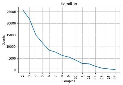
Figure 1: Mendenhall’s curve for Hamilton.
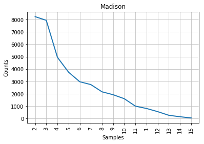
Figure 2: Mendenhall’s curve for Madison.
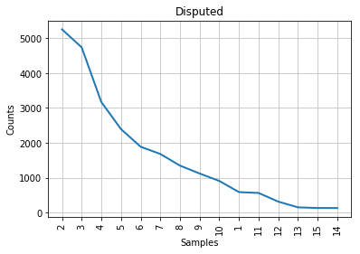
Figure 3: Mendenhall’s curve for the disputed papers.
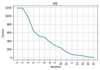
Figure 4: Mendenhall’s curve for Jay.
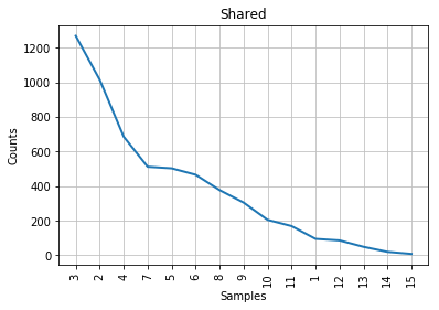
Figure 5: Mendenhall’s curve for the papers co-authored by Madison and Hamilton.
As you can see from the graphs, the characteristic curve associated with the disputed papers looks like a compromise between Madison’s and Hamilton’s. The leftmost part of the disputed papers’ graph, which accounts for the most frequent word lengths, looks a bit more similar to Madison’s; the tail end of the graph, like Hamilton’s. This is consistent with the historical observation that Madison and Hamilton had similar styles, but it does not help us much with our authorship attribution task. The best that we can say is that John Jay almost certainly did not write the disputed papers, because his curve looks nothing like the others; lengths 6 and 7 are even inverted in his part of the corpus, compared to everyone else’s.
If we had no additional information to work with, we would tend to conclude that the disputed papers are probably Madison’s work, albeit without much confidence. Fortunately, stylometric science has advanced a great deal since Mendenhall’s time.
Second Stylometric Test: Kilgariff’s Chi-Squared Method
In a 2001 paper, Adam Kilgarriff15 recommends using the chi-squared statistic to determine authorship. Readers familiar with statistical methods may recall that chi-squared is sometimes used to test whether a set of observations (say, voters’ intentions as stated in a poll) follow a certain probability distribution or pattern. This is not what we are after here. Rather, we will simply use the statistic to measure the “distance” between the vocabularies employed in two sets of texts. The more similar the vocabularies, the likelier it is that the same author wrote the texts in both sets. This assumes that a person’s vocabulary and word usage patterns are relatively constant.
Here is how to apply the statistic for authorship attribution:
- Take the corpora associated with two authors.
- Merge them into a single, larger corpus.
- Count the tokens for each of the words that can be found in this larger corpus.
- Select the
nmost common words in the larger corpus. - Calculate how many tokens of these
nmost common words we would have expected to find in each of the two original corpora if they had come from the same author. This simply means dividing the number of tokens that we have observed in the combined corpus into two values, based on the relative sizes of the two authors’ contributions to the common corpus. -
Calculate a chi-squared distance by summing, over the
nmost common words, the squares of the differences between the actual numbers of tokens found in each author’s corpus and the expected numbers, divided by the expected numbers. Figure 6 shows the equation for the chi-squared statistic, where C(i) represents the observed number of tokens for feature ‘i’, and E(i), the expected number for this feature.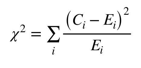
Figure 6: Equation for the chi-squared statistic.
The smaller the chi-squared value, the more similar the two corpora. Therefore, we will calculate a chi-squared for the difference between the Madison and Disputed corpora, and another for the difference between the Hamilton and Disputed corpora; the smaller value will indicate which of Madison and Hamilton is the most similar to Disputed.
Note: No matter which stylometric method we use, the choice of n, the number of words to take into consideration, is something of a dark art. In the literature surveyed by Stamatatos2, scholars have suggested between 100 and 1,000 of the most common words; one project even used every word that appeared in the corpus at least twice. As a guideline, the larger the corpus, the larger the number of words that can be used as features without running the risk of giving undue importance to a word that occurs only a handful of times. In this lesson, we will use a relatively large n for the chi-squared method and a smaller one for the next method. Changing the value of n will certainly change the numeric results a little; however, if a small modification of n causes a change in authorship attribution, this is a sign that the test you are performing is unable to provide meaningful evidence regarding your test case.
The following code snippet implements Kilgariff’s method, with the frequencies of the 500 most common words in the joint corpus being used in the calculation:
# Who are the authors we are analyzing?
authors = ("Hamilton", "Madison")

# Lowercase the tokens so that the same word, capitalized or not,
# counts as one word
for author in authors:
    federalist_by_author_tokens[author] = (
        [token.lower() for token in federalist_by_author_tokens[author]])
federalist_by_author_tokens["Disputed"] = (
    [token.lower() for token in federalist_by_author_tokens["Disputed"]])

# Calculate chisquared for each of the two candidate authors
for author in authors:

    # First, build a joint corpus and identify the 500 most frequent words in it
    joint_corpus = (federalist_by_author_tokens[author] +
                    federalist_by_author_tokens["Disputed"])
    joint_freq_dist = nltk.FreqDist(joint_corpus)
    most_common = list(joint_freq_dist.most_common(500))

    # What proportion of the joint corpus is made up
    # of the candidate author's tokens?
    author_share = (len(federalist_by_author_tokens[author])
                    / len(joint_corpus))

    # Now, let's look at the 500 most common words in the candidate
    # author's corpus and compare the number of times they can be observed
    # to what would be expected if the author's papers
    # and the Disputed papers were both random samples from the same distribution.
    chisquared = 0
    for word,joint_count in most_common:

        # How often do we really see this common word?
        author_count = federalist_by_author_tokens[author].count(word)
        disputed_count = federalist_by_author_tokens["Disputed"].count(word)

        # How often should we see it?
        expected_author_count = joint_count * author_share
        expected_disputed_count = joint_count * (1-author_share)

        # Add the word's contribution to the chi-squared statistic
        chisquared += ((author_count-expected_author_count) *
                       (author_count-expected_author_count) /
                       expected_author_count)

        chisquared += ((disputed_count-expected_disputed_count) *
                       (disputed_count-expected_disputed_count)
                       / expected_disputed_count)

    print("The Chi-squared statistic for candidate", author, "is", chisquared)
The output produced by the chi-squared method should look like this:
The Chi-squared statistic for candidate Hamilton is 3434.6850314768426
The Chi-squared statistic for candidate Madison is 1907.5992915766838
As we can see from the above results, the chi-squared distance between the Disputed and Hamilton corpora is considerably larger than the distance between the Madison and Disputed corpora. This is a strong sign that, if a single author is responsible for the 12 papers in the Disputed corpus, that author is Madison rather than Hamilton.
However, chi-squared is still a coarse method. For one thing, words that appear very frequently tend to carry a disproportionate amount of weight in the final calculation. Sometimes this is fine; other times, subtle differences in style represented by the ways in which authors use more unusual words will go unnoticed.
A Note about Parts of Speech
In some languages, it may be useful to apply parts-of-speech tagging to the word tokens before counting them, so that the same word used as two different parts of speech may count as two different features. For example, in French, very common words like “la” and “le” serve both as articles (in which case they would translate into English as “the”) and as pronouns (“it”). This lesson does not use part-of-speech tagging because it is rarely useful for stylometric analysis in contemporary English and because nltk’s default tagger does not support other languages very well.
Should you need to apply part-of-speech tagging to your own data, you may be able to download taggers for other languages, to work with a third-party tool like Tree Tagger, or even to train your own tagger, but these techniques are far beyond the scope of the current lesson.
Third Stylometric Test: John Burrows’ Delta Method (Advanced)
The first two stylometric methods were easy to implement. This next one, based on John Burrows’ Delta statistic16, is considerably more involved, both conceptually (the mathematics are more complicated) and computationally (more code required). It is, however, one of the most prominent stylometric methods in use today.
Like Kilgariff’s chi-squared, Burrows’ Delta is a measure of the “distance” between a text whose authorship we want to ascertain and some other corpus. Unlike chi-squared, however, the Delta Method is designed to compare an anonymous text (or set of texts) to many different authors’ signatures at the same time. More precisely, Delta measures how the anonymous text and sets of texts written by an arbitrary number of known authors all diverge from the average of all of them put together. Furthermore, the Delta Method gives equal weight to every feature that it measures, thus avoiding the problem of common words overwhelming the results, which was an issue with chi-squared tests. For all of these reasons, John Burrows’ Delta Method is usually a more effective solution to the problem of authorship.
Burrows’ original algorithm can be summarized as follows:
- Assemble a large corpus made up of texts written by an arbitrary number of authors; let’s say that number of authors is
x. - Find the
nmost frequent words in the corpus to use as features. - For each of these
nfeatures, calculate the share of each of thexauthors’ subcorpora represented by this feature, as a percentage of the total number of words. As an example, the word “the” may represent 4.72% of the words in Author A’s subcorpus. - Then, calculate the mean and the standard deviation of these
xvalues and use them as the offical mean and standard deviation for this feature over the whole corpus. In other words, we will be using a mean of means instead of calculating a single value representing the share of the entire corpus represented by each word. This is because we want to avoid a larger subcorpus, like Hamilton’s in our case, over-influencing the results in its favor and defining the corpus norm in such a way that everything would be expected to look like it. -
For each of the
nfeatures andxsubcorpora, calculate az-scoredescribing how far away from the corpus norm the usage of this particular feature in this particular subcorpus happens to be. To do this, subtract the “mean of means” for the feature from the feature’s frequency in the subcorpus and divide the result by the feature’s standard deviation. Figure 7 shows the z-score equation for feature ‘i’, where C(i) represents the observed frequency, the greek letter mu represents the mean of means, and the greek letter sigma, the standard deviation.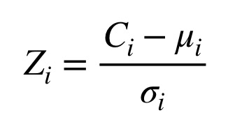
Figure 7: Equation for the z-score statistic.
- Then, calculate the same
z-scoresfor each feature in the text for which we want to determine authorship. -
Finally, calculate a delta score comparing the anonymous paper with each candidate’s subcorpus. To do this, take the average of the absolute values of the differences between the
z-scoresfor each feature between the anonymous paper and the candidate’s subcorpus. (Read that twice!) This gives equal weight to each feature, no matter how often the words occur in the texts; otherwise, the top 3 or 4 features would overwhelm everything else. Figure 8 shows the equation for Delta, where Z(c,i) is the z-score for feature ‘i’ in candidate ‘c’, and Z(t,i) is the z-score for feature ‘i’ in the test case.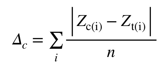
Figure 8: Equation for John Burrows’ Delta statistic.
- The “winning” candidate is the author for whom the delta score between the author’s subcorpus and the test case is the lowest.
Stefan Evert et al.17 provide an in-depth discussion of the method’s variants, refinements and intricacies, but we will stick to the essentials for the purposes of this lesson. A different explanation of Delta, written in Spanish, and an application to a corpus of Spanish novels can also be found in a recent paper by José Calvo Tello.18
Our Test Case
As our test case, we will use Federalist 64. Alexander Hamtilton claimed to be the author of this paper in his letter; however, a draft of Federalist 64 was later found in John Jay’s personal papers and everyone concluded that Jay was in fact the author. No foul play is suspected, by the way: in the same letter, Hamilton attributed to Jay the authorship of another paper with a similar number that Hamilton himself had clearly written. Perhaps Hamilton was distracted by his pending duel and simply misremembered.
Since John Burrows’ Delta Method works with an arbitrary number of candidate authors (Burrows’ original paper uses about 25), we will compare Federalist 64’s stylistic signature with those of five corpora: Hamilton’s papers, Madison’s papers, Jay’s other papers, the papers co-written by Madison and Hamilton, and the papers disputed between Hamilton and Madison. We expect the Delta Method to tell us that Jay is the most likely author; any other result would call into question either the method, or the historiography, or both.
Feature Selection
Let’s combine all of the subcorpora into a single corpus for Delta to calculate a “standard” to work with. Then, let’s select a number of words to use as features. Remember that we used 500 words to calculate Kilgariff’s chi-squared; this time, we will use a smaller set of 30 words, most if not all of them function words and common verbs, as our features.
# Who are we dealing with this time?
authors = ("Hamilton", "Madison", "Jay", "Disputed", "Shared")

# Convert papers to lowercase to count all tokens of the same word together
# regardless of case
for author in authors:
    federalist_by_author_tokens[author] = (
        [tok.lower() for tok in federalist_by_author_tokens[author]])

# Combine every paper except our test case into a single corpus
whole_corpus = []
for author in authors:
    whole_corpus += federalist_by_author_tokens[author]

# Get a frequency distribution
whole_corpus_freq_dist = list(nltk.FreqDist(whole_corpus).most_common(30))
whole_corpus_freq_dist[ :10 ]
A sample of the most frequent words with their frequency occurence looks like this:
[('the', 17846),
('of', 11796),
('to', 7012),
('and', 5016),
('in', 4408),
('a', 3967),
('be', 3370),
('that', 2747),
('it', 2520),
('is', 2178)]
Calculating features for each subcorpus
Let’s look at the frequencies of each feature in each candidate’s subcorpus, as a proportion of the total number of tokens in the subcorpus. We’ll calculate these values and store them in a dictionary of dictionaries, a convenient way of building a two-dimensional array in Python.
# The main data structure
features = [word for word,freq in whole_corpus_freq_dist]
feature_freqs = {}

for author in authors:
    # A dictionary for each candidate's features
    feature_freqs[author] = {}

    # A helper value containing the number of tokens in the author's subcorpus
    overall = len(federalist_by_author_tokens[author])

    # Calculate each feature's presence in the subcorpus
    for feature in features:
        presence = federalist_by_author_tokens[author].count(feature)
        feature_freqs[author][feature] = presence / overall
Calculating feature averages and standard deviations
Given the feature frequencies for all four subcorpora that we have just computed, we can find a “mean of means” and a standard deviation for each feature. We’ll store these values in another “dictionary of dictionaries”.
import math

# The data structure into which we will be storing the "corpus standard" statistics
corpus_features = {}

# For each feature...
for feature in features:
    # Create a sub-dictionary that will contain the feature's mean
    # and standard deviation
    corpus_features[feature] = {}

    # Calculate the mean of the frequencies expressed in the subcorpora
    feature_average = 0
    for author in authors:
        feature_average += feature_freqs[author][feature]
    feature_average /= len(authors)
    corpus_features[feature]["Mean"] = feature_average

    # Calculate the standard deviation using the basic formula for a sample
    feature_stdev = 0
    for author in authors:
        diff = feature_freqs[author][feature] - corpus_features[feature]["Mean"]
        feature_stdev += diff*diff
    feature_stdev /= (len(authors) - 1)
    feature_stdev = math.sqrt(feature_stdev)
    corpus_features[feature]["StdDev"] = feature_stdev
Calculating z-scores
Next, we transform the observed feature frequencies in the five candidates’ subcorpora into z-scores describing how far away from the “corpus norm” these observations are. Nothing fancy here: we merely apply the definition of the z-score to each feature and store the results into yet another two-dimensional array.
feature_zscores = {}
for author in authors:
    feature_zscores[author] = {}
    for feature in features:

        # Z-score definition = (value - mean) / stddev
        # We use intermediate variables to make the code easier to read
        feature_val = feature_freqs[author][feature]
        feature_mean = corpus_features[feature]["Mean"]
        feature_stdev = corpus_features[feature]["StdDev"]
        feature_zscores[author][feature] = ((feature_val-feature_mean) /
                                            feature_stdev)
Calculating features and z-scores for our test case
Next, we need to compare Federalist 64 with the corpus. The following code snippet, which essentially recapitulates everything we have done so far, counts the frequencies of each of our 30 features in Federalist 64 and calculates z-scores accordingly:
# Tokenize the test case
testcase_tokens = nltk.word_tokenize(federalist_by_author["TestCase"])

# Filter out punctuation and lowercase the tokens
testcase_tokens = [token.lower() for token in testcase_tokens
                   if any(c.isalpha() for c in token)]

# Calculate the test case's features
overall = len(testcase_tokens)
testcase_freqs = {}
for feature in features:
    presence = testcase_tokens.count(feature)
    testcase_freqs[feature] = presence / overall

# Calculate the test case's feature z-scores
testcase_zscores = {}
for feature in features:
    feature_val = testcase_freqs[feature]
    feature_mean = corpus_features[feature]["Mean"]
    feature_stdev = corpus_features[feature]["StdDev"]
    testcase_zscores[feature] = (feature_val - feature_mean) / feature_stdev
    print("Test case z-score for feature", feature, "is", testcase_zscores[feature])
The results of some features z-scores for Federalist 64 should look like this (a sample):
Test case z-score for feature the is -0.7692828380408238
Test case z-score for feature of is -1.8167784558461264
Test case z-score for feature to is 1.032705844508835
Test case z-score for feature and is 1.0268752924746058
Test case z-score for feature in is 0.6085448501260903
Test case z-score for feature a is -0.9341289591084886
Test case z-score for feature be is 1.0279650702511498
Calculating Delta
And finally, we use the formula for Delta defined by Burrows to extract a single score comparing Federalist 64 with each of the five “candidate authors”. Reminder: the smaller the Delta score, the more similar Federalist 64’s stylometric signature is to the candidate’s.
for author in authors:
    delta = 0
    for feature in features:
        delta += math.fabs((testcase_zscores[feature] -
                            feature_zscores[author][feature]))
    delta /= len(features)
    print( "Delta score for candidate", author, "is", delta )
The results: Delta scores suggest that John Jay indeed wrote Federalist 64:
Delta score for candidate Hamilton is 1.768470453004334
Delta score for candidate Madison is 1.6089724119682816
Delta score for candidate Jay is 1.5345768956569326
Delta score for candidate Disputed is 1.5371768107570636
Delta score for candidate Shared is 1.846113566619675
As expected, Delta identifies John Jay as Federalist 64’s most likely author. It is interesting to note that, according to Delta, Federalist 64 is more similar to the disputed papers than to those known to have been written by Hamilton or by Madison; why that might be, however, is a question for another day.
Further Reading and Resources
Interesting case studies
Stylometry and/or authorship attribution have been used in many contexts, employing many techniques. Here are but a few interesting case studies:
- Javier de la Rosa and Juan Luis Suárez look for the author or a famous 16th-century Spanish novel from among a considerable list of candidates.19
- Maria Slautina and Mikhail Marusenko use pattern recognition on a set of syntactic, grammatical and lexical features, from simple word counts (with part-of-speech tagging) to various types of phrases, in order to establish stylistic similarity between medieval texts.20
- Ellen Jordan, Hugh Craig and Alexis Antonia look at the case of 19th-century British periodicals, in which articles were usually unsigned, to determine the author of four reviews of works by or about the Brontë sisters.21 This case study applies an early version of another method developed by John Burrows, the Zeta method, which focuses on an author’s favorite words instead of common function words.22
- Valérie Beaudoin and François Yvon analyse 58 plays in verse by French playwrights Corneille, Racine and Molière, finding that the first two were far more consistent in the way they structured their writing than the latter.23
- Marcelo Luiz Brocardo, Issa Traore, Sherif Saad and Isaac Woungang apply supervised learning and n-gram models to determine the authorship of short messages with large numbers of potential authors, like emails and tweets.24
- Moshe Koppel and Winter Yaron propose the “impostor method”, which attempts to determine whether two texts have been written by the same author by inserting them into a set of texts written by false candidates.25 Justin Anthony Stover et al. have recently applied the technique to determine the authorship of a newly discovered 2nd-century manuscript.26
- Finally, a team led by David I. Holmes studies the peculiar case of documents written either by a Civil War soldier or by his widow who may intentionally have copied his writing style.27
Additional references on authorship and stylometry
The most exhaustive reference in all matters related to authorship attribution, including the history of the field, its mathematical and linguistic underpinnings, and its various methods, was written by Patrick Juola in 2007.28 Chapter 7, in particular, shows how authorship attribution can serve as a marker for various group identities (gender, nationality, dialect, etc.), for change in language over time, and even for personality and mental health.
A shorter survey can be found in Moshe Koppel et al., who discuss cases in which there is a single candidate author whose authorship must be confirmed, large numbers of candidates for which only small writing samples are available to train a machine learning algorithm, or no known candidate at all.29
The Stamatatos paper cited earlier2 also contains a quality survey of the field.
Varia
Programming historians who wish to explore stylometry further may want to download the Stylo package30, which has become a de facto standard. Among other things, Stylo provides an implementation of the Delta method, feature extraction functionality, and convenient graphical user interfaces for both data manipulation and the production of visually appealing results. Note that Stylo is written in R, which means that you will need R installed on your computer to run it, but between the graphical user interface and the tutorials, little or no prior knowledge of R programming should be necessary.
Readers fluent in French who are interested in exploring the epistemological implications of the interactions between quantitative and qualitative methods in the analysis of writing style should read Clémence Jacquot.31
Somewhat surprisingly, data obtained through optical character recognition (OCR) have been shown to be adequate for authorship attribution purposes, even when the data suffer from high OCR error rates.32
Readers interested in further discussion of the history of the Federalist Papers and of the various theories advanced regarding their authorship may want to start by reading papers by Irving Brant33 and by Paul Ford and Edward Bourne.34 The topic, however, is almost boundless.
Finally, there is a Zotero group dedicated to stylometry, where you can find many more references to methods and studies.
Acknowledgements
Thanks to Stéfan Sinclair and Andrew Piper, in whose seminars at McGill University this project began. Also thanks to my thesis advisor, Susan Dalton, whose mentorship in always invaluable.
Endnotes
-
See, for example, Justin Rice, “What Makes Hemingway Hemingway? A statistical analysis of the data behind Hemingway’s style” ↩
-
Efstathios Stamatatos, “A Survey of Modern Authorship Attribution Method,” Journal of the American Society for Information Science and Technology, vol. 60, no. 3 (December 2008), p. 538–56, citation on p. 540, https://doi.org/10.1002/asi.21001. ↩ ↩2 ↩3
-
Jan Rybicki, “Vive La Différence: Tracing the (Authorial) Gender Signal by Multivariate Analysis of Word Frequencies,” Digital Scholarship in the Humanities, vol. 31, no. 4 (December 2016), pp. 746–61, https://doi.org/10.1093/llc/fqv023. Sean G. Weidman and James O’Sullivan, “The Limits of Distinctive Words: Re-Evaluating Literature’s Gender Marker Debate,” Digital Scholarship in the Humanities, 2017, https://doi.org/10.1093/llc/fqx017. ↩
-
Ted Underwood, David Bamman, and Sabrina Lee, “The Transformation of Gender in English-Language Fiction”, Cultural Analytics, Feb. 13, 2018, DOI: 10.7910/DVN/TEGMGI. ↩
-
Sven Meyer zu Eissen and Benno Stein, “Intrinsic Plagiarism Detection,” in ECIR 2006, edited by Mounia Lalmas, Andy MacFarlane, Stefan Rüger, Anastasios Tombros, Theodora Tsikrika, and Alexei Yavlinsky, Berlin, Heidelberg: Springer, 2006, pp. 565–69, https://doi.org/10.1007/11735106_66. ↩
-
Cynthia Whissell, “Traditional and Emotional Stylometric Analysis of the Songs of Beatles Paul McCartney and John Lennon,” Computers and the Humanities, vol. 30, no. 3 (1996), pp. 257–65. ↩
-
Douglass Adair, “The Authorship of the Disputed Federalist Papers”, The William and Mary Quarterly, vol. 1, no. 2 (April 1944), pp. 97-122. ↩
-
David I. Holmes and Richard S. Forsyth, “The Federalist Revisited: New Directions in Authorship Attribution”, Literary and Linguisting Computing, vol. 10, no. 2 (1995), pp. 111-127. ↩
-
Frederick Mosteller, “A Statistical Study of the Writing Styles of the Authors of the Federalist Papers”, Proceedings of the American Philosophical Society, vol. 131, no. 2 (1987), pp. 132‑40. ↩
-
Frederick Mosteller and David Lee Wallace, Inference and Disputed Authorship: The Federalist, Addison-Wesley Series in Behavioral Science : Quantitative Methods (Reading, Mass.: Addison-Wesley PublCo, 1964). ↩
-
See for example Glenn Fung, “The disputed Federalist papers: SVM feature selection via concave minimization”, TAPIA ‘03: Proceedings of the 2003 conference on Diversity in Computing, pp. 42-46; and Robert A. Bosch and Jason A. Smith, “Separating Hyperplanes and the Authorship of the Disputed Federalist Papers,” The American Mathematical Monthly, vol. 105, no. 7 (1998), pp. 601–8, https://doi.org/10.2307/2589242. ↩
-
Jeff Collins, David Kaufer, Pantelis Vlachos, Brian Butler and Suguru Ishizaki, “Detecting Collaborations in Text: Comparing the Authors’ Rhetorical Language Choices in The Federalist Papers”, Computers and the Humanities, vol. 38 (2004), pp. 15-36. ↩
-
Mosteller, “A Statistical Study…”, pp. 132-133. ↩
-
T. C. Mendenhall, “The Characteristic Curves of Composition”, Science, vol. 9, no. 214 (Mar. 11, 1887), pp. 237-249. ↩
-
Adam Kilgarriff, “Comparing Corpora”, International Journal of Corpus Linguistics, vol. 6, no. 1 (2001), pp. 97-133. ↩
-
John Burrows, “‘Delta’: a Measure of Stylistic Difference and a Guide to Likely Authorship”, Literary and Linguistic Computing, vol. 17, no. 3 (2002), pp. 267-287. ↩
-
Stefan Evert et al., “Understanding and explaining Delta measures for authorship attribution”, Digital Scholarship in the Humanities, vol. 32, no. suppl_2 (2017), pp. ii4-ii16. ↩
-
José Calvo Tello, “Entendiendo Delta desde las Humanidades,” Caracteres, May 27 2016, http://revistacaracteres.net/revista/vol5n1mayo2016/entendiendo-delta/. ↩
-
Javier de la Rosa and Juan Luis Suárez, “The Life of Lazarillo de Tormes and of His Machine Learning Adversities,” Lemir, vol. 20 (2016), pp. 373-438. ↩
-
Maria Slautina and Mikhaïl Marusenko, “L’émergence du style, The emergence of style,” Les Cahiers du numérique, vol. 10, no. 4 (November 2014), pp. 179–215, https://doi.org/10.3166/LCN.10.4.179-215. ↩
-
Ellen Jordan, Hugh Craig, and Alexis Antonia, “The Brontë Sisters and the ‘Christian Remembrancer’: A Pilot Study in the Use of the ‘Burrows Method’ to Identify the Authorship of Unsigned Articles in the Nineteenth-Century Periodical Press,” Victorian Periodicals Review, vol. 39, no. 1 (2006), pp. 21–45. ↩
-
John Burrows, “All the Way Through: Testing for Authorship in Different Frequency Strata,” Literary and Linguistic Computing, vol. 22, no. 1 (April 2007), pp. 27–47, https://doi.org/10.1093/llc/fqi067. ↩
-
Valérie Beaudoin and François Yvon, “Contribution de La Métrique à La Stylométrie,” JADT 2004: 7e Journées internationales d’Analyse statistique des Données Textuelles, vol. 1, Louvain La Neuve, Presses Universitaires de Louvain, 2004, pp. 107–18. ↩
-
Marcelo Luiz Brocardo, Issa Traore, Sherif Saad and Isaac Woungang, “Authorship Verification for Short Messages Using Stylometry,” 2013 International Conference on Computer, Information and Telecommunication Systems (CITS), 2013, https://doi.org/10.1109/CITS.2013.6705711. ↩
-
Moshe Koppel and Winter Yaron, “Determining If Two Documents Are Written by the Same Author,” Journal of the Association for Information Science and Technology, vol. 65, no. 1 (October 2013), pp. 178–87, https://doi.org/10.1002/asi.22954. ↩
-
Justin Anthony Stover et al., “Computational authorship verification method attributes a new work to a major 2nd century African author”, Journal of the Association for Information Science and Technology, vol. 67, no. 1 (2016), pp. 239–242. ↩
-
David I. Holmes, Lesley J. Gordon, and Christine Wilson, “A widow and her soldier: Stylometry and the American Civil War”, Literary and Linguistic Computing, vol. 16, no 4 (2001), pp. 403–420. ↩
-
Patrick Juola, “Authorship Attribution,” Foundations and Trends in Information Retrieval, vol. 1, no. 3 (2007), pp. 233–334, https://doi.org/10.1561/1500000005. ↩
-
Moshe Koppel, Jonathan Schler, and Shlomo Argamon, “Computational Methods in Authorship Attribution,” Journal of the Association for Information Science and Technology. vol. 60, no. 1 (January 2009), pp. 9–26, https://doi.org/10.1002/asi.v60:1. ↩
-
Maciej Eder, Jan Rybicki, and Mike Kestemont, “Stylometry with R: A Package for Computational Text Analysis,” The R Journal, vol. 8, no. 1 (2016), pp. 107–21. ↩
-
Clémence Jacquot, “Rêve d’une épiphanie du style: visibilité et saillance en stylistique et en stylométrie,” Revue d’Histoire Littéraire de la France , vol. 116, no. 3 (2016), pp. 619–39. ↩
-
Patrick Juola, John Noecker Jr, and Michael Ryan, “Authorship Attribution and Optical Character Recognition Errors”, TAL, vol. 53, no. 3 (2012), pp. 101–127. ↩
-
Irving Brant, “Settling the Authorship of the Federalist”, The American Historical Review, vol. 67, no. 1 (October 1961), pp. 71-75. ↩
-
Paul Leicester Ford and Edward Gaylord Bourne, “The Authorship of the Federalist”, The American Historical Review, vol. 2, no. 4 (July 1897), pp. 675-687. ↩