Contents
- Introduction
- Learning Objectives
- Prerequisites
- Installing FFmpeg
- Basic Structure and Syntax of FFmpeg commands
- Getting Started
- Preliminary Command Examples
- Wrap Up
- References
Introduction
The Digital Humanities, as a discipline, have historically focused almost exclusively on the analysis of textual sources through computational methods (Hockey, 2004). However, there is growing interest in the field around using computational methods for the analysis of audiovisual cultural heritage materials as indicated by the creation of the Alliance of Digital Humanities Organizations Special Interest Group: Audiovisual Materials in the Digital Humanities and the rise in submissions related to audiovisual topics at the global ADHO conference over the past few years. Newer investigations, such as Distant Viewing TV, also indicate a shift in the field toward projects concerned with using computational techniques to expand the scope of materials digital humanists can investigate. As Erik Champion states, “The DH audience is not always literature-focused or interested in traditional forms of literacy,” and applying digital methodologies to the study of audiovisual culture is an exciting and emerging facet of the discipline (Champion, 2017). There are many valuable, free, and open-source tools and resources available to those interested in working with audiovisual materials (for example, the Programming Historian tutorial Editing Audio with Audacity), and this tutorial will introduce another: FFmpeg.
FFmpeg is “the leading multimedia framework able to decode, encode, transcode, mux, demux, stream, filter, and play pretty much anything that humans and machines have created” (FFmpeg Website - “About”). Many common software applications and websites use FFmpeg to handle reading and writing audiovisual files, including VLC, Google Chrome, YouTube, and many more. In addition to being a software and web-developer tool, FFmpeg can be used at the command-line to perform many common, complex, and important tasks related to audiovisual file management, alteration, and analysis. These kinds of processes, such as editing, transcoding (re-encoding), or extracting metadata from files, usually require access to other software (such as a non-linear video editor like Adobe Premiere or Final Cut Pro), but FFmpeg allows a user to operate on audiovisual files directly without the use of third-party software or interfaces. As such, knowledge of the framework empowers users to manipulate audiovisual materials to meet their needs with a free, open-source solution that carries much of the functionality of expensive audio and video editing software. This tutorial will provide an introduction to reading and writing FFmpeg commands and walk through a use-case for how the framework can be used in Digital Humanities scholarship (specifically, how FFmpeg can be used to extract and analyze color data from an archival video source).
Learning Objectives
- Install FFmpeg on your computer or use a demo version in your web browser
- Understand the basic structure and syntax of FFmpeg commands
- Execute several useful commands such as:
- Re-wrapping (change file container) & Transcoding (re-encode files)
- Demuxing (separating audio and video tracks)
- Trimming/Editing files
- File playback with FFplay
- Creating vectorscopes for color data visualization
- Generating color data reports with FFprobe
- Introduce outside resources for further exploration and experimentation
Prerequisites
Before starting this tutorial, you should be comfortable with locating and using your computer’s Terminal or other command-line interface, as this is where you will be entering and executing FFmpeg commands. If you need instruction on how to access and work at the command-line, I recommend the Program Historian’s Bash tutorial for Mac and Linux users or the Windows PowerShell tutorial. Additionally, a basic understanding of audiovisual codecs and containers will also be useful to understanding what FFmpeg does and how it works. We will provide some additional information and discuss codecs and containers in a bit more detail in the Preliminary Command Examples section of this tutorial.
Installing FFmpeg
Installing FFmpeg can be the most difficult part of using FFmpeg. Thankfully, there are some helpful guides and resources available for installing the framework based on your operating system.
For Mac OS Users
The simplest option is to use a package manager such as Homebrew to install FFmpeg and ensure it remains in the most up-to-date version. Homebrew is also useful in ensuring that your computer has the necessary dependencies installed to ensure FFMpeg runs properly. To complete this kind of installation, follow these steps:
- Install Homebrew following the instructions in the above link
- You can then run
brew install ffmpegin your Terminal to initiate a basic installation.- Note: Generally, it is recommended to install FFMpeg with additional features than what is included in the basic installation. Including additional options will provide access to more of FFmpeg’s tools and functionalities. Reto Kromer’s Apple installation guide provides a good set of additional options:
brew install ffmpeg --with-sdl2 --with-freetype --with-openjpeg --with-x265 --with-rubberband --with-tesseract- For an explanation of these additional options, refer to Ashley Blewer’s FFmpeg guide
- Additionally, you can run
brew options ffmpegto see what features are or have become available with the current FFmpeg release
-
After installing, it is best practice to update Homebrew and FFmpeg to ensure all dependencies and features are most up-to-date by running:
brew update && brew upgrade ffmpeg - For more installation options for Mac OS, see the Mac OS FFmpeg Compilation Guide
For Windows Users
Windows users can use the package manager Chocolately to install and maintain FFmpeg. Reto Kromer’s Windows installation guide provides all the necessary information to use Chocolately or to install the software from a build.
For Linux Users
Linuxbrew, a program similar to Homebrew, can be used to install and maintain FFmpeg in Linux. Reto Kromer also provides a helpful Linux installation guide that closely resembles the Mac OS installation. Your distribution of Linux may also have its own package manager already installed that include FFmpeg packages available. Depending on your distribution of Linux (Ubuntu, Fedora, Arch Linux, etc.) these builds can vary, so using Linuxbrew could be useful to ensure that the build is the same regardless of which type of Linux you are using.
Other Installation Resources
- Download Packages
- FFmpeg allows access to binary files, source code, and static builds for Mac, Windows, and Linux directly through its website, enabling users to build the framework without a package manager. It is likely that only advanced users will want to follow this option.
- FFmpeg Compilation Guide
- The FFmpeg Wiki page also provides a compendium of guides and strategies for building FFmpeg on your computer.
Testing the Installation
-
To ensure FFmpeg is installed properly, run:
ffmpeg -version -
If you see a long output of information, the installation was successful! It should look similar to this:
ffmpeg version 4.0.1 Copyright (c) 2000-2018 the FFmpeg developers built with Apple LLVM version 9.1.0 (clang-902.0.39.1) configuration: --prefix=/usr/local/Cellar/ffmpeg/4.0.1 --enable-shared --enable-pthreads --enable-version3 --enable-hardcoded-tables --enable-avresample --cc=clang --host-cflags= --host-ldflags= --enable-gpl --enable-ffplay --enable-libfreetype --enable-libmp3lame --enable-librubberband --enable-libtesseract --enable-libx264 --enable-libx265 --enable-libxvid --enable-opencl --enable-videotoolbox --disable-lzma --enable-libopenjpeg --disable-decoder=jpeg2000 --extra-cflags=-I/usr/local/Cellar/openjpeg/2.3.0/include/openjpeg-2.3 libavcodec 58. 18.100 / 58. 18.100 libavformat 58. 12.100 / 58. 12.100 libavdevice 58. 3.100 / 58. 3.100 libavfilter 7. 16.100 / 7. 16.100 libavresample 4. 0. 0 / 4. 0. 0 libswscale 5. 1.100 / 5. 1.100 libswresample 3. 1.100 / 3. 1.100 libpostproc 55. 1.100 / 55. 1.100 -
If you see something like
-bash: ffmpeg: command not foundthen something has gone wrong.- Note: If you are using a package manager it is unlikely that you will encounter this error message. However, if there is a problem after installing with a package manager, it is likely the issue is with the package manager itself as opposed to FFmpeg. Consult the Troubleshooting sections for Homebrew, Chocolatey, or Linuxbrew to ensure the package manager is functioning properly on your computer. If you are attempting to install without a package manager and see this error message, cross-reference your method with the FFmpeg Compilation Guide provided above.
Using FFmpeg in a web browser (without installing)
If you do not want to install FFmpeg on your computer but would like to become familiar with using it at the command-line, Brian Grinstead’s videoconverter.js provides a way to run FFmpeg commands and learn its basic functions in the web-browser of your choice.
Basic Structure and Syntax of FFmpeg commands
Basic FFmepg commands consist of four elements:
[Command Prompt] [Input File] [Flags/Actions] [Output File]
- A command prompt will begin every FFmpeg command. Depending on the use, this prompt will either be
ffmpeg(changing files),ffprobe(gathering metadata from files), orffplay(playback of files). - Input files are the files being read, edited, or examined.
- Flags and actions are the things you are telling FFmpeg to do the input files. Most commands will contain multiple flags and actions of various complexity.
- The output file is the new file created by the command or the report generated by an
ffprobecommand.
Written generically, a basic FFmpeg command looks like this:
ffmpeg -i /filepath/input_file.ext -flag some_action /filepath/output_file.ext
Next, we will look at some examples of several different commands that use this structure and syntax. These commands will also demonstrate some of FFmpeg’s most basic, useful functions and allow us to become more familiar with how digital audiovisual files are constructed.
Getting Started
For this tutorial, we will be taking an archival film called Destination Earth as our object of study. This film has been made available by the Prelinger Archives collection on the Internet Archive. Released in 1956, this film is a prime example of Cold War-era propaganda produced by the American Petroleum Institute and John Sutherland Productions that extols the virtues of capitalism and the American way of life. Utilizing the Technicolor process, this science-fiction animated short tells a story of a Martian society living under an oppressive government and their efforts to improve their industrial methods. They send an emissary to Earth who discovers the key to this is oil refining and free-enterprise. We will be using this video to introduce some of the basic functionalities of FFmpeg and analyzing its color properties in relation to its propagandist rhetoric.

Destination Earth (1956)
For this tutorial, you will need to:
- Navigate to the Destination Earth page on IA
- Download two video files: the “MPEG4” (file extension
.m4v) and “OGG” (file extension.ogv) versions of the film - Save these two video files in the same folder somewhere on your computer. Save them with the file names
destEarthfollowed by its extension
Take a few minutes to watch the video and get a sense of its structure, message, and visual motifs before moving on with the next commands.
Preliminary Command Examples
Viewing Basic Metadata with FFprobe
Before we begin manipulating our destEarth files, let’s use FFmpeg to examine some basic information about the file itself using a simple ffprobe command. This will help illuminate how digital audiovisual files are constructed and provide a foundation for the rest of the tutorial. Navigate to the file’s directory and execute:
ffprobe destEarth.ogv
You will see the file’s basic technical metadata printed in the stdout:
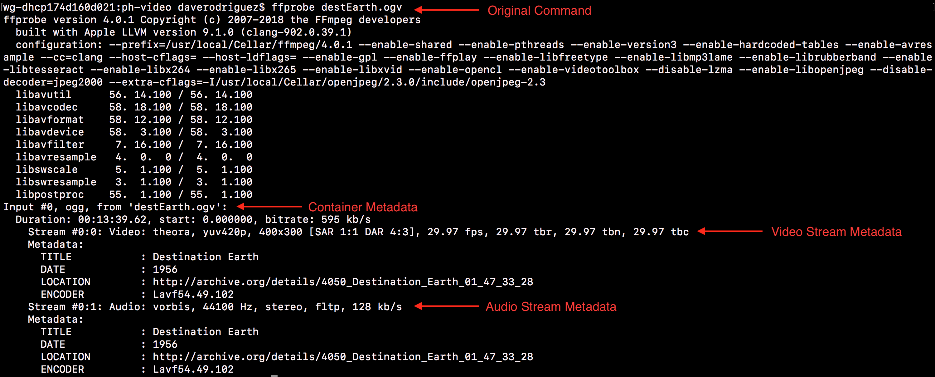
The output of a basic ffprobe command with destEarth.ogv
The Input #0 line of the reports identifies the container as ogg. Containers (also called “wrappers”) provide the file with structure for its various streams. Different containers (other common ones include .mkv, .avi, and .flv) have different features and compatibilities with various software. We will examine how and why you might want to change a file’s container in the next command.
The lines Stream #0:0 and Stream #0:1 provide information about the file’s streams (i.e. the content you see on screen and hear through your speakers) and identify the codec of each stream as well. Codecs specify how information is encoded/compressed (written and stored) and decoded/decompressed (played back). Our .ogv file’s video stream (Stream #0:0) uses the theora codec while the audio stream (Stream #0:1) uses the vorbis codec. These lines also provide important information related to the video stream’s colorspace (yuv420p), resolution (400x300), and frame-rate (29.97 fps), in addition to audio information such as sample-rate (44100 Hz) and bit-rate (128 kb/s).
Codecs, to a much greater extent than containers, determine an audiovisual file’s quality and compatibility with different software and platforms (other common codecs include DNxHD and ProRes for video and mp3 and FLAC for audio). We will examine how and why you might want to change a file’s codec in the next command as well.
Run another ffprobe command, this time with the .m4v file:
ffprobe destEarth.m4v
Again you’ll see the basic technical metadata printed to the stdout:
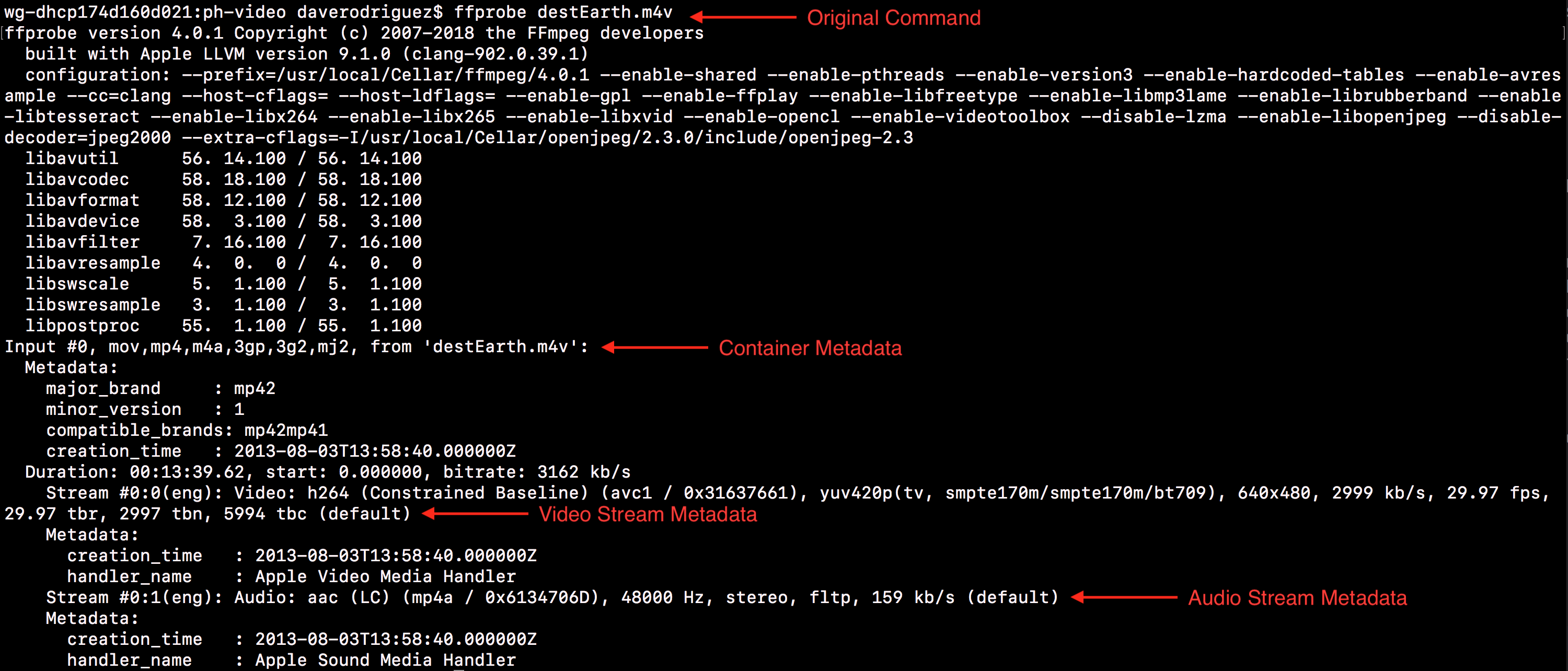
The output of a basic ffprobe command with destEarth.m4v
You’ll also notice that the report for the .m4v file contains multiple containers on the Input #0 line like mov and m4a. It isn’t necessary to get too far into the details for the purposes of this tutorial, but be aware that the mp4 and mov containers come in many “flavors” and different file extensions. However, they are all very similar in their technical construction, and as such you may see them grouped together in technical metadata. Similarly, the ogg file has the extension .ogv, a “flavor” or variant of the ogg format.
Just as in our previous command, the lines Stream #0:0 and Stream #0:1 identify the codec of each stream. We can see our .m4v file uses the H.264 video codec while the audio stream uses the aac codec. Notice that we are given similar metadata to our .ogv file but some important features related to visual analysis (such as the resolution) are significantly different. Our .m4v has a much higher resolution (640x480) and we will therefore use this version of Destination Earth as our source video.
Now that we know more about the technical make-up of our file, we can begin exploring the transformative features and functionalities of FFmpeg (we will use ffprobe again later in the tutorial to conduct more advanced color metadata extraction).
Changing Containers and Codecs (Re-Wrap and Transcode)
Depending on your operating system, you may have one or more media players installed. For the purposes of demonstration, let’s see what happens if you try to open destEarth.ogv using the QuickTime media player that comes with Mac OSX:
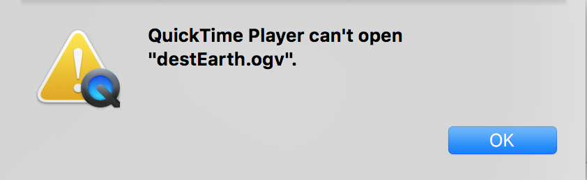
Proprietary media players such as QuickTime are often limited in the kinds of files they can work with.
One option when faced with such a message is to simply use another media player. VLC, which is built with FFmpeg, is an excellent open-source alternative, but simply “using another software” may not always be a viable solution (and you may not always have another version of a file to work with, either). Many popular video editors such as Adobe Premiere, Final Cut Pro, and DaVinci Resolve all have their own limitations on the kinds of formats they are compatible with. Further, different web-platforms and hosting/streaming sites such as Vimeo have their own requirements as well. As such, it is important to be able to re-wrap and transcode your files to meet the various specifications for playback, editing, digital publication, and conforming files to standards required by digital preservation or archiving platforms.
ffmpeg -codecs and ffmpeg -formats, respectively, to see the list printed to your stdout.
As an exercise in learning basic FFmpeg syntax and learning how to transcode between formats, we will begin with our destEarth.ogv file and write a new file with video encoded to H.264, audio to AAC, and wrapped in an .mp4 container, a very common and highly-portable combination of codecs and container that is practically identical to the .m4v file we originally downloaded. Here is the command you will execute along with an explanation of each part of the syntax:
ffmpeg -i destEarth.ogv -c:v libx264 -c:a aac destEarth_transcoded.mp4
ffmpeg= starts the command-i destEarth.ogv= specifies the input file-c:v libx264= transcodes the video stream to the H.264 codec-c:a aac= transcodes the audio stream to the AAC codecdestEarth_transcoded.mp4= specifies the output file. Note this is where the new container type is specified.
If you execute this command as it is written and in the same directory as destEarth.ogv, you will see a new file called destEarth_transcoded.mp4 appear in the directory. If you are operating in Mac OSX, you will also be able to play this new file with QuickTime. A full exploration of codecs, containers, compatibility, and file extension conventions is beyond the scope of this tutorial, however this preliminary set of examples should give those less familiar with how digital audiovisual files are constructed a baseline set of knowledge that will enable them to complete the rest of the tutorial.
Creating Excerpts & Demuxing Audio & Video
Now that we have a better understanding of streams, codecs, and containers, let’s look at ways FFmpeg can help us work with video materials at a more granular level. For this tutorial, we will examine two discrete sections of Destination Earth to compare how color is used in relation to the film’s propagandist rhetoric. We will create and prepare these excerpts for analysis using a command that performs two different functions simultaneously:
- First, the command will create two excerpts from
destEarth.m4v. - Second, the command will remove (“demux”) the audio components (
Stream #0:1) from these excerpts.We are removing the audio in the interest of promoting good practice in saving storage space (the audio information is not necessary for color analysis). This will likely be useful if you hope to use this kind of analysis at larger scales. More on scaling color analysis will be provided near the end of the tutorial.
The first excerpt we will be making is a sequence near the beginning of the film depicting the difficult conditions and downtrodden life of the Martian society. The following command specifies start and end points of the excerpt, tells FFmpeg to retain all information in the video stream without transcoding anything, and to write our new file without the audio stream:
ffmpeg -i destEarth.m4v -ss 00:01:00 -to 00:04:35 -c:v copy -an destEarth_Mars_video.mp4
ffmpeg= starts the command-i destEarth.m4v= specifies the input file-ss 00:01:00= sets start point at 1 minute from start of file-to 00:04:45= sets end point to 4 minutes and 45 seconds from start of file-c:v copy= copy the video stream directly, without transcoding-an= tells FFmpeg to ignore audio stream when writing the output file.-
destEarth_Mars_video.mp4= specifies the output file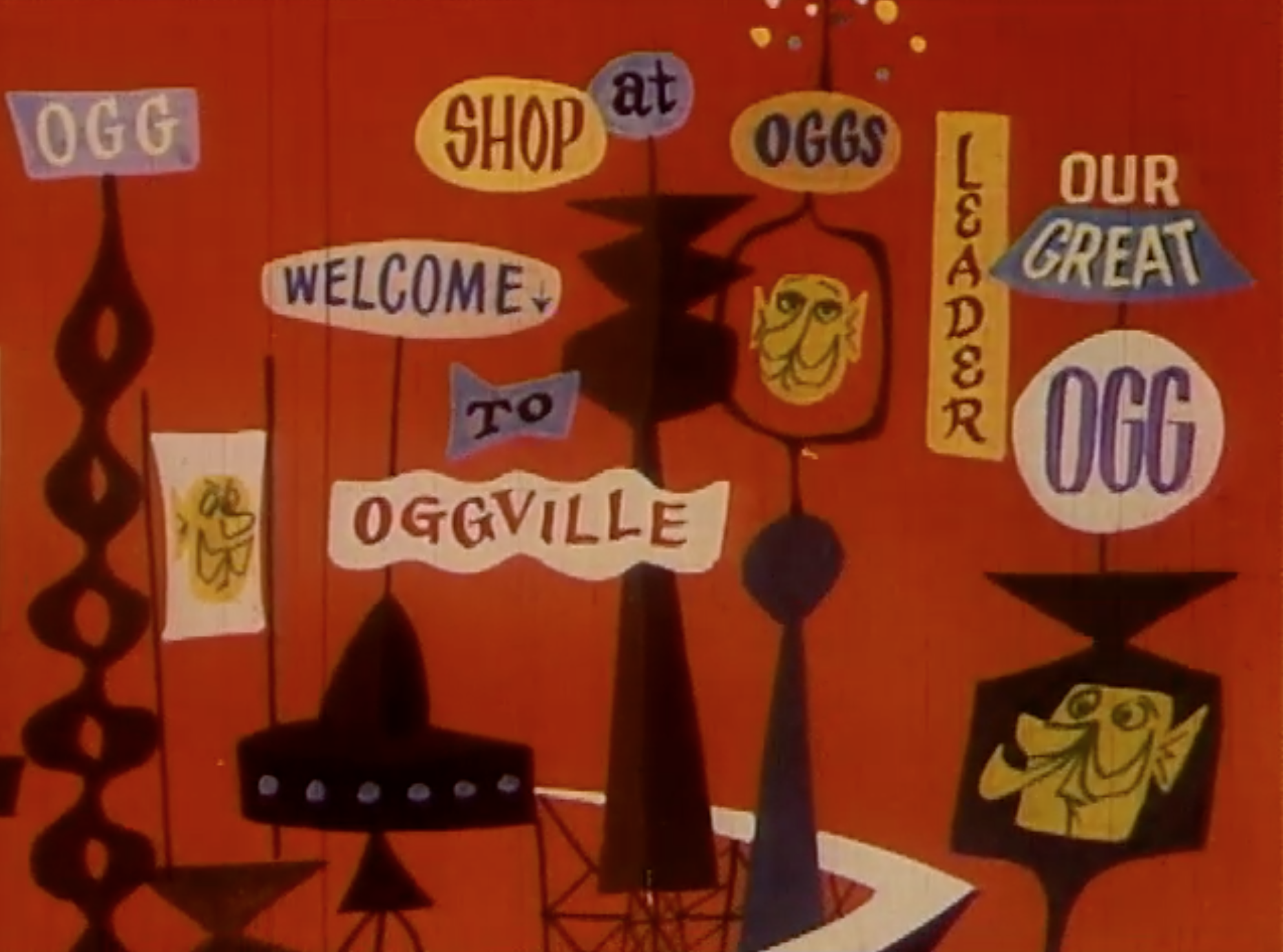
Life on Mars
We will now run a similar command to create an “Earth” excerpt. This portion of the film has a similar sequence depicting the wonders of life on Earth and the richness of its society thanks to free-enterprise capitalism and the use of oil and petroleum products:
ffmpeg -i destEarth.m4v -ss 00:07:30 -to 00:11:05 -c:v copy -an destEarth_Earth_video.mp4
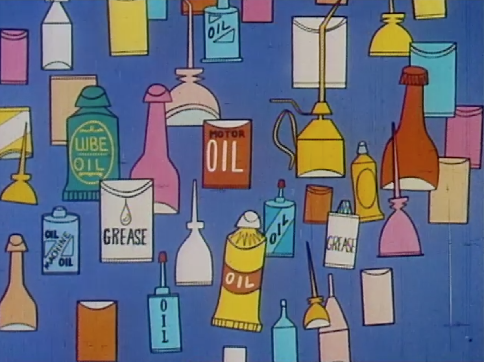
Bounty of Earth
You should now have two new files in your directory called destEarth_Mars_video.mp4 and destEarth_Earth_video.mp4. You can test one or both files (or any of the other files in the directory) using the ffplay feature of FFmpeg as well. Simply run:
ffplay destEarth_Mars_video.mp4
and/or
ffplay destEarth_Earth_video.mp4
You will see a window open and the video will begin at the specified start point, play through once, and then close (in addition, you’ll notice there is no sound in your video). You will also notice that ffplay commands do not require an -i or an output to be specified because the playback itself is the output.
FFplay is a very versatile media player that comes with a number of options for customizing playback. For example, adding `-loop 0` to the command will loop playback indefinitely.We have now created our two excerpts for analysis. If we watch these clips discretely, there appear to be significant, meaningful differences in the way color and color variety are used. In the next part of the tutorial, we will examine and extract data from the video files to quantify and support this hypothesis.
Color Data Analysis
The use of digital tools to analyze color information in motion pictures is another emerging facet of DH scholarship that overlaps with traditional film studies. The FilmColors project, in particular, at the University of Zurich, interrogates the critical intersection of film’s “formal aesthetic features to [the] semantic, historical, and technological aspects” of its production, reception, and dissemination through the use of digital analysis and annotation tools (Flueckiger, 2017). Although there is no standardized method for this kind of investigation at the time of this writing, the ffprobe command offered below is a powerful tool for extracting information related to color that can be used in computational analysis. First, let’s look at another standardized way of representing color information that informs this quantitative, data-driven approach to color analysis.
Vectorscopes
For years, video professionals have relied on vectorscopes to view color information in a standardized and easily legible way. A vectorscope plots color information on a circular graticle, and the position of a given plot corresponds to the particular hues found in a video signal. Other factors, like saturation, determine the size of a given plot as well. Below is an example of a vectorscope displaying the color values of SMPTE Bars, which are also pictured.
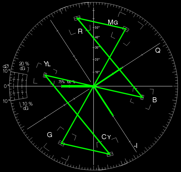
A vectorscope read-out representing standard NTSC SMPTE Bars. Source: Wikimedia Commons

NTSC SMPTE Bars. Source: Wikimedia Commons
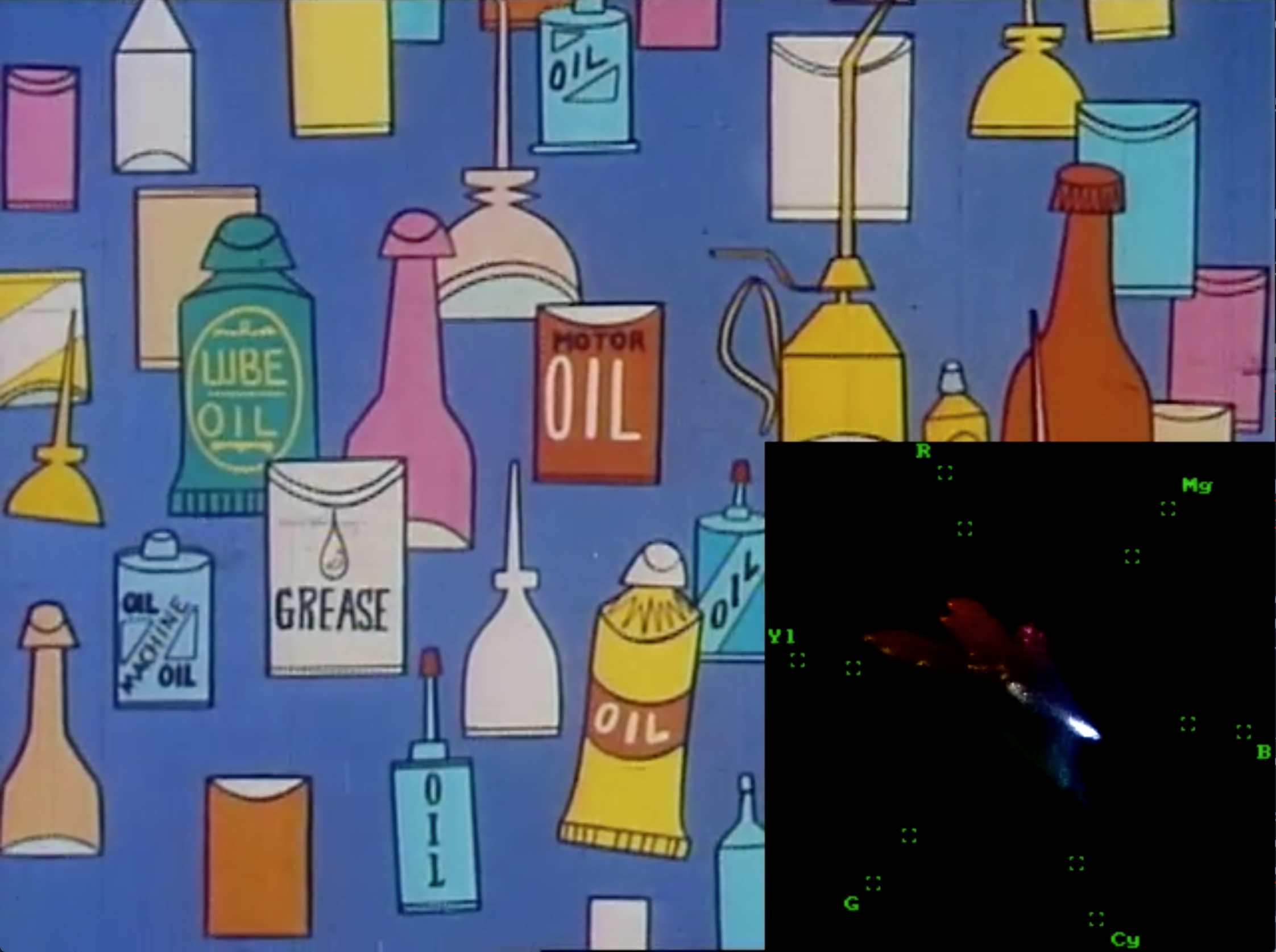
FFmpeg can be used to playback and create video files with vectorscopes embedded in them so as to provide a real-time reference for the video’s color information. The following ffplay commands will embed a vectorscope in the lower-right corner of the frame. As the video plays, you will notice the vectorscope plot shift as the on-screen color shifts:
ffplay destEarth_Mars_video.mp4 -vf "split=2[m][v], [v]vectorscope=b=0.7:m=color3:g=green[v],[m][v]overlay=x=W-w:y=H-h"
ffplay= starts the commanddestEarth_Mars_video.mp4= specifies the input file-vf= creates a filter-graph to use for the streams"= quotation mark to start the filter-graph. Information inside the quotation marks will specify the parameters of the vectorscope’s appearance and position.split=2[m][v]= splits the input into two identical outputs called[m]and[v],= comma signifies another parameter is coming[v]vectorscope=b=0.7:m=color3:g=green[v]= assigns the[v]output the vectorscope filter. Thebflag specifies the vectorscope’s background opacity, themflag the vectorscope mode, and thegflag the color of the graticle.[m][v]overlay=x=W-w:y=H-h= overlays the vectorscope on top of the video image (the[m]output) in a certain location determined by x:y coordinates. In this case, the vectorscope will be justified to the lower right corner of the frame."= ends the filter-graph
Screenshot of FFplay window with embedded vectorscope
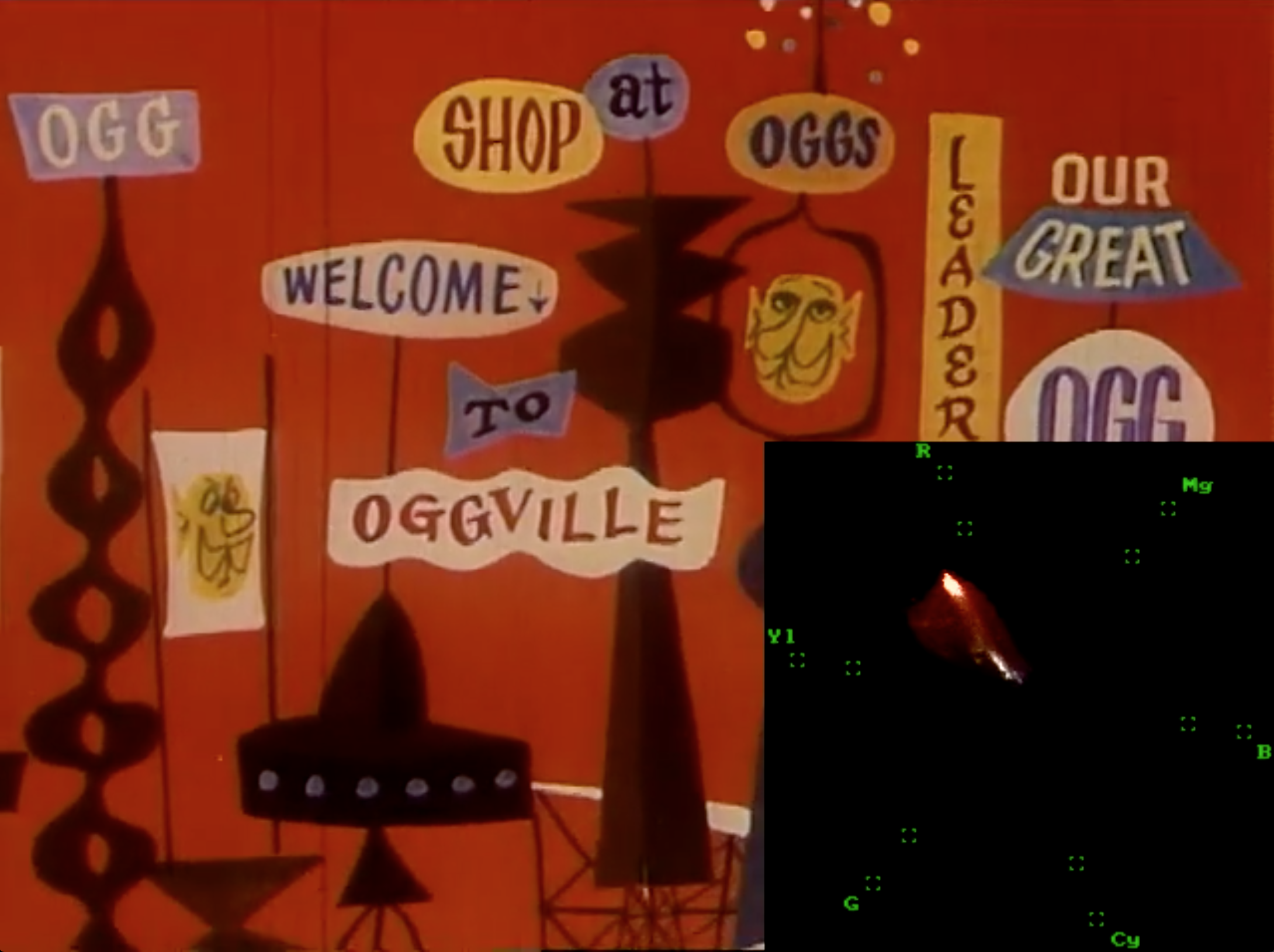
And for the “Earth” excerpt:
ffplay destEarth_Earth_video.mp4 -vf "split=2[m][v], [v]vectorscope=b=0.7:m=color3:g=green[v],[m][v]overlay=x=W-w:y=H-h"
Screenshot of FFplay window with embedded vectorscope
We can also adjust this command to write new video files with vectorscopes as well:
ffmpeg -i destEarth_Mars_video.mp4 -vf "split=2[m][v], [v]vectorscope=b=0.7:m=color3:g=green[v],[m][v]overlay=x=W-w:y=H-h" -c:v libx264 destEarth_Mars_vectorscope.mp4
ffmpeg -i destEarth_Earth_video.mp4 -vf "split=2[m][v], [v]vectorscope=b=0.7:m=color3:g=green[v],[m][v]overlay=x=W-w:y=H-h" -c:v libx264 destEarth_Earth_vectorscope.mp4
Note the slight but important changes in syntax:
- We have added an
-iflag because it is anffmpegcommand. - We have specified the output video codec as H.264 with the flag
-c:v libx264and have left out an option for audio. Although you could add-c:a copyto copy the audio stream (if there is one in the input file) without transcoding or specify another audio codec here if necessary. - We have specified the name of the output file.
Take a few minutes to watch these videos with the vectorscopes embedded in them. Notice how dynamic (or not) the changes are between the “Mars” and “Earth” excerpts. Compare what you see in the vectorscope to your own impressions of the video itself. We might use observations from these vectorscopes to make determinations about which shades of color appear more regularly or intensely in a given source video, or we may compare different formats side-by-side to see how color gets encoded or represented differently based on different codecs, resolutions, etc.
Although vectorscopes provide a useful, real-time representation of color information, we may want to also access the raw data beneath them. We can then use this data to develop more flexible visualizations that are not dependent on viewing the video file simultaneously and that offer a more quantitative approach to color analysis. In our next commands, we will use ffprobe to produce a tabular dataset that can be used to create a graph of color data.
Color Data Extraction with FFprobe
At the beginning of this tutorial, we used an ffprobe command to view our file’s basic metadata printed to the stdout. In these next examples, we’ll use ffprobe to extract color data from our video excerpts and output this information to .csv files. Within our ffprobe command, we are going to use the signalstats filter to create .csv reports of median color hue information for each frame in the video stream of destEarth_Mars_video.mp4 and destEarth_Earth_video.mp4, respectively.
ffprobe -f lavfi -i movie=destEarth_Mars_video.mp4,signalstats -show_entries frame=pkt_pts_time:frame_tags=lavfi.signalstats.HUEMED -print_format csv > destEarth_Mars_hue.csv
ffprobe= starts the command-f lavfi= specifies the libavfilter virtual input device as the chosen format. This is necessary when usingsignalstatsand many filters in more complex FFmpeg commands.-i movie=destEarth_Mars_video.mp4= name of input file,signalstats= specifies use of thesignalstatsfilter with the input file-show_entries= sets list of entries that will be shown in the report. These are specified by the next options.frame=pkt_pts_time= specifies showing each frame with its correspondingpkt_pts_time, creating a unique entry for each frame of video:frame_tags=lavfi.signalstats.HUEMED= creates a tag for each frame that contains the median hue value-print_format csv= specifies the format of the metadata report> destEarth_Mars_hue.csv= writes a new.csvfile containing the metadata report using>, a Bash redirection operator. Simply, this operator takes the command the precedes it and “redirects” the output to another location. In this instance, it is writing the output to a new.csvfile. The file extension provided here should also match the format specified by theprint_formatflag
Next, run the same command for the “Earth” excerpt:
ffprobe -f lavfi -i movie=destEarth_Earth_video.mp4,signalstats -show_entries frame=pkt_pts_time:frame_tags=lavfi.signalstats.HUEMED -print_format csv > destEarth_Earth_hue.csv
signalstats filter and the various metrics that can be extracted from video streams, refer to the FFmpeg's Filters Documentation.
You should now have two .csv files in your directory. If you open these in a text editor or spreadsheet program, you will see three columns of data:
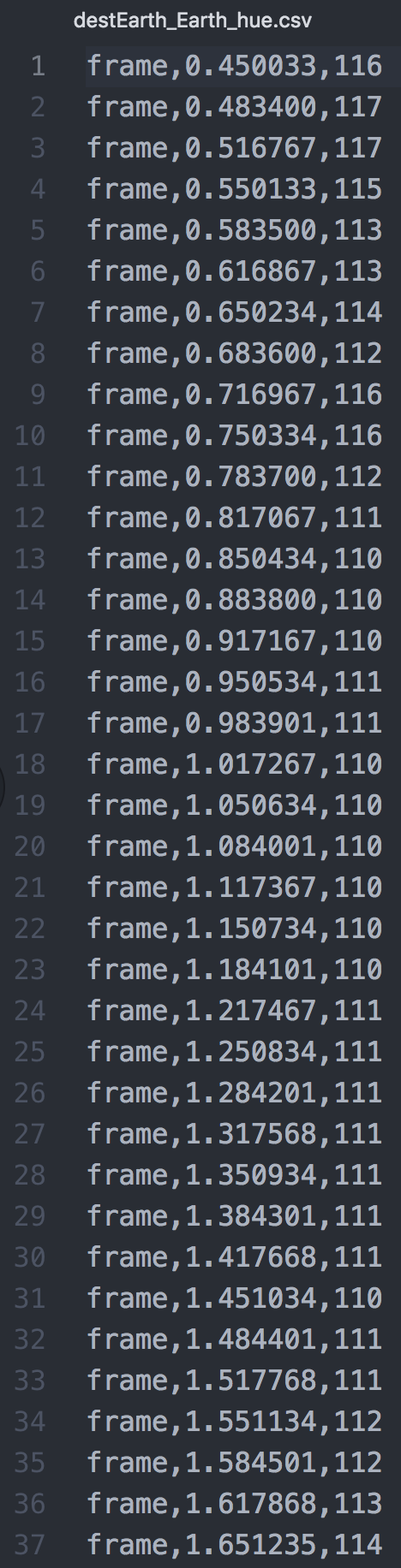
The first several rows of our Earth excerpt color report in .csv format
Going from left to right, the first two columns give us information about where we are in the video. The decimal numbers represent fractions of a second that also roughly correspond to the video’s time-base of 30fps. As such, each row in our .csv corresponds to one frame of video. The third column carries a whole number between 0-360, and this value represents the median hue for that frame of video. These numbers are the underlying quantitative data of the vectorscope’s plot and correspond to its position (in radians) on the circular graticle. Referencing our vectorscope image from earlier, you can see that starting at the bottom of the circle (0 degrees) and moving left, “greens” are around 38 degrees, “yellows” at 99 degrees, “reds” at 161 degrees, “magentas” at 218 degrees, “blues” at 279 degrees, and “cyans” at 341 degrees. Once you understand these “ranges” of hue, you can get an idea of what the median hue value for a given video frame is just by looking at this numerical value.
Additionally, It is worth noting that this value extracted by the signalstats filter is not an absolute or complete measure of an image’s color qualities, but simply a meaningful point of reference from which we can explore a data-driven approach to color analysis. Color perception and color theory are complex, evolving areas of scholarly investigation that incorporate many different approaches from the humanities, social sciences, and cognitive sciences. As such, we should be mindful that any analytical approach should be taken within the context of these larger discourses and with a collaborative and generative spirit.
Graphing Color Data
The two .csv files we created with the previous commands can now be used to create graphs visualizing the data. There are a number of platforms (both proprietary and open-source) that can be used to achieve this such as Microsoft Excel, RAWGraphs, and/or plot.ly. An in-depth discussion of how to use any of these platforms is outside the scope of this tutorial, however, the final visualization of the previous commands (below) was created by uploading the .csv files to plot.ly, an open-source, browser-based service that offers a number of tutorials on how to use their platform.
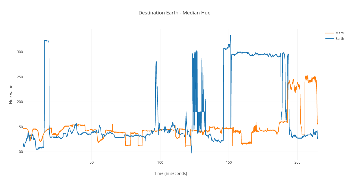
Graph including median hue data from both video excerpts
Conclusions
From looking at the graph, we can see that the Mars and Earth traces have very different dynamic ranges in their median hue values. The Mars trace is very limited and keeps within the red and yellow ranges (roughly between 100 - 160) throughout the majority of the excerpt. This suggests something about the film’s use of color as a rhetorical device serving a propagandist message. Remember that this section presents an antipathetic view of the Martian way of life and political system: a uniform, unhappy populace who are dependent on inefficient technology and transportation while being required to observe total obedience to a totalitarian overlord. The film connects this negative experience to a relatively dull color palette of reds and yellows. We should also consider the original target audience of this film, young citizens of the United States in the 1950s, and how they would have likely interpreted these images and uses of color in that historical moment, namely, in the context of increasing geopolitical tensions between the Soviet Union and the United States and its allies in Western Europe. The color red, specifically, was commonly used in print and broadcast media for describing the “threat” of global Communism during this era of world history. Additionally, the choice to render the Martian totalitarian leader with a very similar appearance to iconic Soviet leader Joseph Stalin can be read as an explicit visual and cultural cue to the audience. As such, this depiction of Mars seems to be a thinly-veiled allegorical caricature of life under Communism as perceived by an outside observer and political/ideological opponent, a caricature that employs not only a limited color palette but one that is charged with other cultural references. The use of color both leverages the preconceived biases and associations of its audience and is inherently bound to the film’s political argument that Communism is not a viable or desirable system of government.
Contrasting the limited use of color in our Mars excerpt, the Earth trace covers a much wider dynamic range of hue values. In this passage, the Martian emissary is learning about the wonderful and affluent lifestyle of Earthlings thanks to a capitalist system and exploitation of oil and petroleum products. The sequence emphasizes the material wealth and entrepreneurial freedom offered under a capitalist system using a much greater variety and vivacity of color than in the Mars excerpt. Commercial products and people alike are depicted using the full spectrum of the Technicolor process, creating positive associations between the outputs of the petroleum industry and the well-off lifestyle of those who benefit from it. Like the Mars excerpt, the audience is offered a one-sided caricature of a political system and way of life, but in this section the reductionist portrayal is laudable and prosperous as opposed to bleak and oppressive. As a piece of propaganda, Destination Earth relies on these powerful but overly simplistic distinctions between two political systems to influence public opinion and promote the consumption of petroleum products. How color is used (or not used) is an important tool in crafting and driving this message home. Further, once we are able to extract color data and visualize it using simple graphing techniques, we can see that the disparity in dynamic range provides a quantitative measure for linking the technical and aesthetic use of color in this animated film with the propagandist rhetoric put forth by its producers.
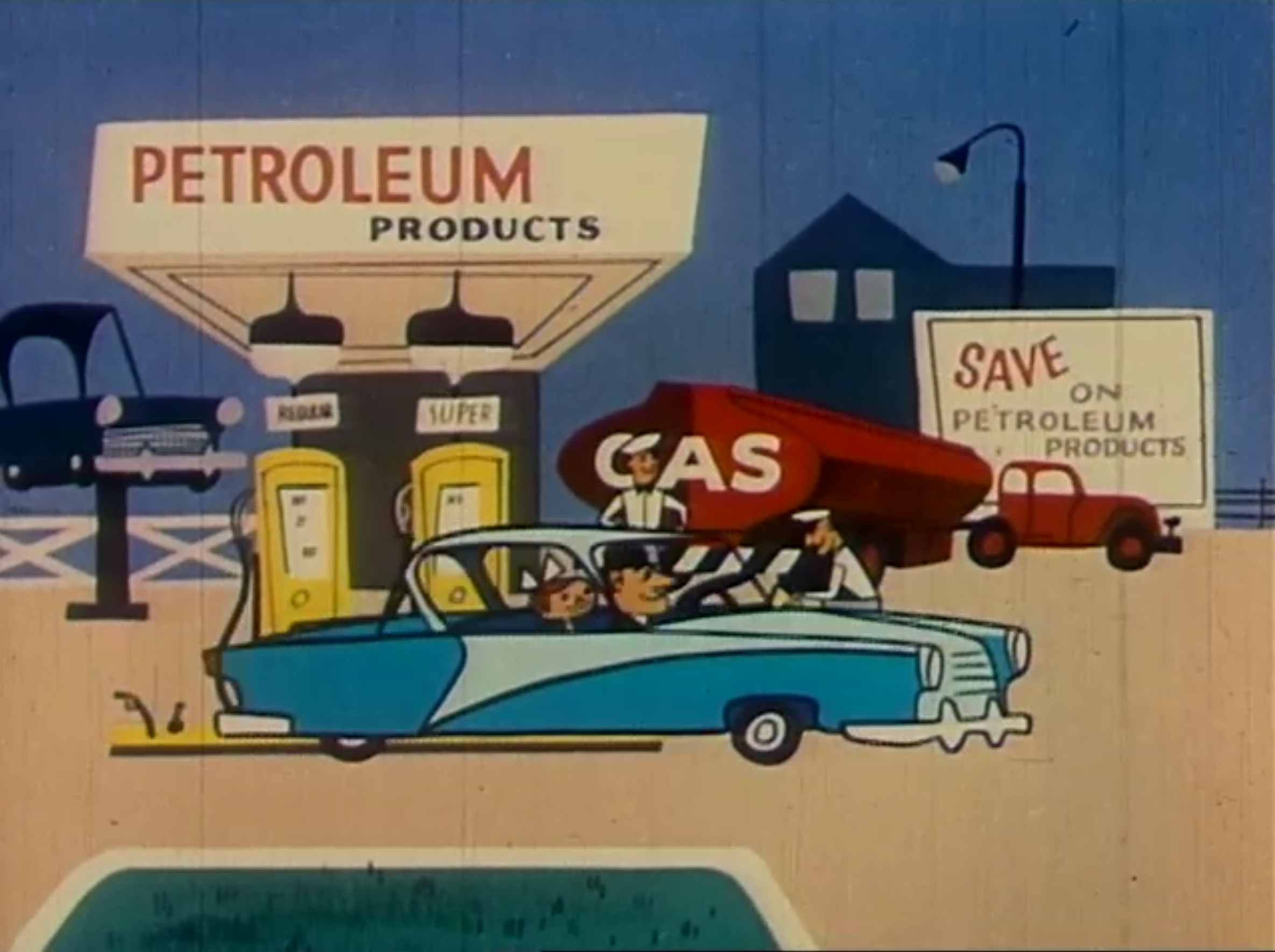
Oil and American ideals of wealth and prosperity rendered in colorful splendor
Scaling Color Analysis with FFprobe
One of the limits of this methodology is that we are manually generating color reports on only one file at a time. If we wanted to take a distant viewing approach more in-line with traditional DH methodologies, we could employ a Bash script to run our ffprobe command on all files in a given directory. This is useful if, for example, a researcher was interested in conducting similar analysis on all the John Sutherland animated films found in the Prelinger Archives collection or another set of archival video material.
Once you have a set of material to work with saved in one place, you can save the following Bash for loop within the directory and execute it to generate .csv files containing the same frame-level median hue data we extracted from our excerpts of Destination Earth.
for file in *.m4v; do
ffprobe -f lavfi -i movie="$file",signalstats -show_entries frame=pkt_pts_time:frame_tags=lavfi.signalstats.HUEMED -print_format csv > "${file%.m4v}.csv";
done
for file in *.m4v; do= initiates the for loop. This first line basically tells FFmpeg: “for all files in this directory with the extension.m4v, perform the following command.”ffprobe -f lavfi -i movie="$file",signalstats -show_entries frame=pkt_pts_time:frame_tags=lavfi.signalstats.HUEMED -print_format csv > "${file%.m4v}.csv"; done= the same color metadata extraction command we ran on our two excerpts of Destination Earth, with some slight alterations to the syntax to account for its use across multiple files in a directory:"$file"recalls each variable. The enclosing quotation marks ensures that the original filename is retained.> "${file%.m4v}.csv";retains the original filename when writing the output.csvfiles. This will ensure the names of the original video files will match their corresponding.csvreports.done= terminates the script once all files in the directory have been looped
signalstats to pull other valuable information related to color. Refer to the filter's documentation for a complete list of visual metrics available.
Once you run this script, you will see each video file in the directory now has a corresponding .csv file containing the specified dataset.
Wrap Up
In this tutorial, we have learned:
- To install FFmpeg on different operating systems and how to access the framework in the web-browser
- The basic syntax and structure of FFmpeg commands
- To view basic technical metadata of an audiovisual file
- To transform an audiovisual file through transcoding and re-wrapping
- To parse and edit that audiovisual file by demuxing it and creating excerpts
- To playback audiovisual files using
ffplay - To create new video files with embedded vectorscopes
- To export tabular data related to color from a video stream using
ffprobe - To craft a Bash for loop to extract color data information from multiple video files with one command
At a broader level, this tutorial aspires to provide an informed and enticing introduction to how audiovisual tools and methodologies can be incorporated in Digital Humanities projects and practices. With open and powerful tools like FFmpeg, there is vast potential for expanding the scope of the field to include more rich and complex types of media and analysis than ever before.
Further Resources
FFmpeg has a large and well-supported community of users across the globe. As such, there are many open-source and free resources for discovering new commands and techniques for working with audio-visual media. Please contact the author with any additions to this list, especially educational resources in Spanish for learning FFmpeg.
- The Official FFmpeg Documentation
- FFmpeg Wiki
- ffmprovisr from the Association of Moving Image Archivists
- Ashley Blewer’s Audiovisual Preservation Training
- Andrew Weaver’s Demystifying FFmpeg
- Ben Turkus’ FFmpeg Presentation
- Reto Kromer’s FFmpeg Cookbook for Archivists
Open-Source AV Analysis Tools using FFmpeg
References
-
Champion, E. (2017) “Digital Humanities is text heavy, visualization light, and simulation poor,” Digital Scholarship in the Humanities 32(S1), i25-i32.
-
Flueckiger, B. (2017). “A Digital Humanities Approach to Film Colors”. The Moving Image, 17(2), 71-94.
-
Hockey, S. (2004) “The History of Humanities Computing,” A Companion to Digital Humanities, ed. Susan Schreibman, Ray Siemens, John Unsworth. Oxford: Blackwell.