Contents
- The Historical Problem & Mathematical Solution
- The Need for a Tutorial
- Lesson Requirements
- The Historical Case Study
- Regression Modelling, and the Mathematics Behind the Model
- The Three Steps of Gravity Modelling
- Taking Your Knowledge Forward
- Acknowledgements
- Endnotes
The Historical Problem & Mathematical Solution
For every 1,000 migrants who moved to London in the 1770s-80s, how many would we expect to come from each English county? For every 1,000 tons of coffee exported from Colombia in 1950, how much would we expect to go to each of the Western Hemisphere’s 21 independent countries?
Both of these historical questions are about movements - people or goods - and are concerned with the resultant distribution from those movements. There are many ways to answer these types of questions, the simplest of which is to assume uniform distribution (25.64 migrants per county, or 47.61 tons of coffee per country). But this is unlikely to be accurate.
Standardising by population may improve accuracy of estimates. How many migrants there were per 10,000 inhabitants? Or how many pounds of coffee was imported per person? While better, it does not provide the full picture because other forces are influencing the outcome (Figure 1). In the first example, the English county of Westmorland had a relatively small population (38,000), and it was also quite far from London (365km). Because of this and other factors, it was unlikely to send as many migrants to London as Berkshire, which had more people (102,000) and was proximal (62km). Population and distance from London were almost certainly factors affecting the number of migrants.
For coffee exports, population is also important. In 1950, the population of Canada (14 million) and the United States (152 million) meant that it was unlikely that they imported the same amount of coffee. Nevertheless, with no domestic supply and a strong coffee-drinking culture, Canada and the United States probably had more in common than they do with many South and Central American countries, who grew their own coffee and had less need to import it. So population, coffee culture, and domestic supply are all relevant variables, as are other factors (Figure 1).
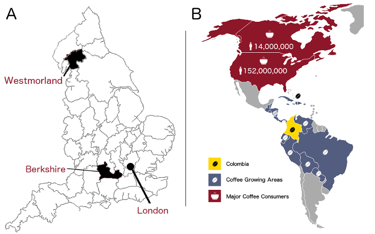
Figure 1: Example A - A map of historic English counties, showing Westmorland, Berkshire, and London. It would be unlikely for both counties to send the same number of migrants to London given differences in population and distance from the capital. Example B - Some of the countries are coffee-producing, and that would affect their need to import, skewing the distribution. Meanwhile, population varies widely between countries. ‘person’ icon by Jens Tärning, ‘Coffee Bean’ by Abdo, ‘Cup’ by alvianwijaya, all from the Noun Project.
To arrive at a more realistic distribution, the approach must take into account several relevant influencing factors. One such approach is a “gravity model”, a mathematical formula based on regression analysis and probability theory that incorporates relevant push, pull, or economic factors into consideration when suggesting a probable distribution between the various territories.
The term “gravity” invokes the idea of forces pulling entities together, as in Isaac Newton’s falling apple. In that case, the relevant factors for calculating gravitational pull were the mass of the apple, the mass of the earth, and the distance between the two. Assuming environmental factors are constant, the apple will always experience the same gravitational pull (or close enough for our purposes). This “universal” law of gravity is represented mathematically by a simple formula:
\[F = G \frac{m_{1}m_{2}}{r_{2}}\]A gravity model of migration or trade is similar in its aim (seeking to understand and measure the forces influencing movement), but is unable to attain the same degree of reliability or repeatability because it measures the results of a series of unpredictable human decisions based on free will rather than the laws of physics. The model is fairly good at predicting how populations will act, but any number of things could influence individual decisions, meaning that the resultant distribution will always be somewhat unpredictable. If you could re-run a realistic migration simulation, you would always end up with slightly different results because you can never account for every relevant variable. Nor do you necessarily want to. The goal is not to build an overly deterministic view of migration or trade, but to get enough information about the key influences to have a historical conversation about meaningful patterns and unexpected discoveries.
So gravitational pull and gravity models are different. As physics is dependable and humans are not, the formula for gravitational pull is simple algebra, whereas the one for gravity modelling of migration or trade draws upon probability theory and is thus part of a different branch of mathematics. Despite this, the term “gravity” is a useful reminder that this approach is about understanding the forces that influence movement.
If you also know how many migrants did come from each county, or now much coffee did go to each nation, the model allows you to identify regional anomalies by comparing the estimated to the observed values. Those might be regions that, given the various contributing factors, were sending more or fewer migrants than we would expect, or consuming disproportionately more or less coffee. These anomalies can then become the subject of scholarly investigation, leading to historical conclusions.
The Need for a Tutorial
While popular with some geographers and economists, and while gravity models have tremendous potential for historians, they have as yet been used very rarely in historical studies. The author was only able to identify two historical migration studies that employed a gravity model as an integral part of the analysis:
-
A.A. Lovett, I.D. Whyte, and K.A. Whyte, “Poisson regression analysis and migration fields: the example of the apprenticeship records of Edinburgh in the seventeenth and eighteenth centuries”, Transactions of the Institute of British Geographers, 10 (1985), pp. 317–32.
-
Adam Crymble, Adam Dennett, Tim Hitchcock, “Modelling regional imbalances in English plebeian migration to late eighteenth-century London”, Economic History Review, 71, 3 (2018), pp. 747-771: https://doi.org/10.1111/ehr.12569.
Given the lack of exposure historians have to gravity models, this tutorial seeks to provide an accessible introduction by providing a walk-through of the example used in my article listed immediately above. This approach allows the reader to try a working gravity model, with the aim of understanding what it is and how it is put together, while also being able to turn to the published literature to see how the modelling process led to scholarly findings.
Lesson Requirements
Software
You will require the following software:
- R programming language
- MASS package for R
- Spreadsheet (Excel or Open Office)
- a scientific calculator (or online equivalent)
The R programming language is a specialist language designed for statistical work. MASS is an add-on code package for R that allows us to conduct certain advanced statistical processes very efficiently. MASS is short for “Modern Applied Statistics with S” and was written in 2002 by William Venables and Brian Ripley. There are many sets of instructions online for how to install R and R packages, including Taryn Dewar’s tutorial on R Basics with Tabular Data.
The tutorial also uses a spreadsheet programme, and a scientific calculator or software or a website that can replicate one. Your calculator should have at least the options highlighted yellow in Figure 2.
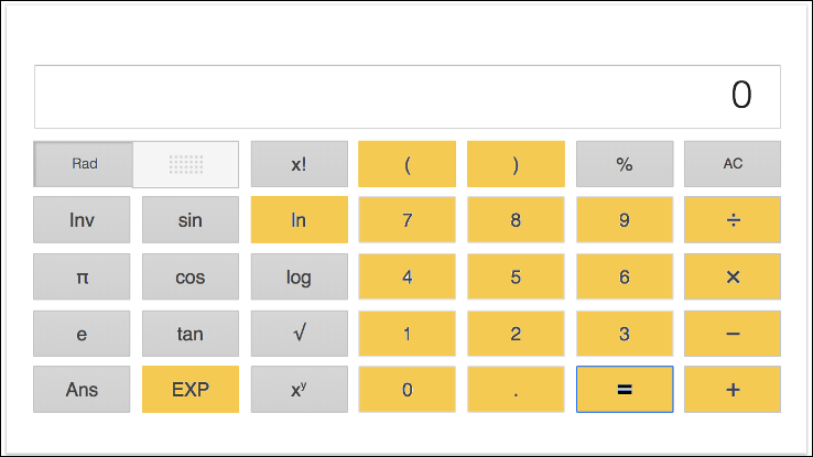
Figure 2: The Google calculator, with the keys used in this tutorial highlighted in yellow. You can use any calculator that has these keys as a minimum.
The associated material for use in this tutorial is introduced as needed. You can also download it all here:
Mathematical Concepts
This tutorial uses a number of mathematical concepts and operations. To understand a gravity model and how it works, you will have to become comfortable with the following concepts and mathematical operations (though it is possible to follow along without all of this knowledge):
- Cartesian coordinates
- exponential function
- mean
- natural logarithm
- order of operations
- Pearson’s correlation coefficient
- probability distribution
- regression analysis
- slope
- square root
- standard deviation
- y-intercept
The Historical Case Study
While gravity models can be used in a range of different migration and trade studies, this tutorial uses a specific historical case study of migration based on the history of vagrancy in eighteenth century London as an example for readers to follow. The materials used in this case study are built from:
1 - Adam Crymble, Adam Dennett, Tim Hitchcock, “Modelling regional imbalances in English plebeian migration to late eighteenth-century London”, Economic History Review, 71, 3 (2018), pp. 747-771: https://doi.org/10.1111/ehr.12569 (Paywall until July 2019).
2 - Adam Crymble, Louise Falcini, Tim Hitchcock, “Vagrant Lives: 14,789 Vagrants Processed by the County of Middlesex, 1777-1786”, Journal of Open Humanities Data, vol. 1, no. 1 (2015), http://doi.org/10.5334/johd.1.
The Vagrancy Act of 1744 gave communities in England and Wales the right to expel outsiders back from whence they came. This was an important right because welfare was distributed locally at the time, and it was paid for by local taxes with the intention of supporting local people. That meant that a large influx of poor outsiders could financially cripple communities that attracted a lot of migration (such as those in London). This restriction on internal migration was only really used against the poor, and constables and local magistrates had tremendous powers of discretion over who they labelled a “vagrant” and who they left alone. As of the time of writing, a version of this law is still on the books in England, and it is still used by the police to arrest people who are begging or who they otherwise feel need to be removed from a situation. People in the late eighteenth century who were arrested under the 1744 act are therefore evidence of internal migration between the various counties of England and London. The question is: were any counties sending more or fewer vagrants to London than we would expect?
This example will model the probable distribution of 3,262 lower-class migrants to London between 1777 and 1786. These “vagrants” were probably visibly poor, but not necessarily to the degree of beggarliness or homelessness. All of them were forcibly expelled from London under the 1744 Vagrancy Act, and sent back to their place of origin.1 They represent a group of failed migrants to the city, and understanding their distribution means we can identify which parts of England sent proportionately higher numbers of vagrants to London. In turn this can help us to understand which parts of the country were under economic stress.
A sample of the primary sources that detail these individuals’ journeys can be seen in Figure 3. At the time of their expulsion from London, each vagrant had his or her name and place of origin recorded, providing a unique account of the lives of thousands of failed migrants to the London area.
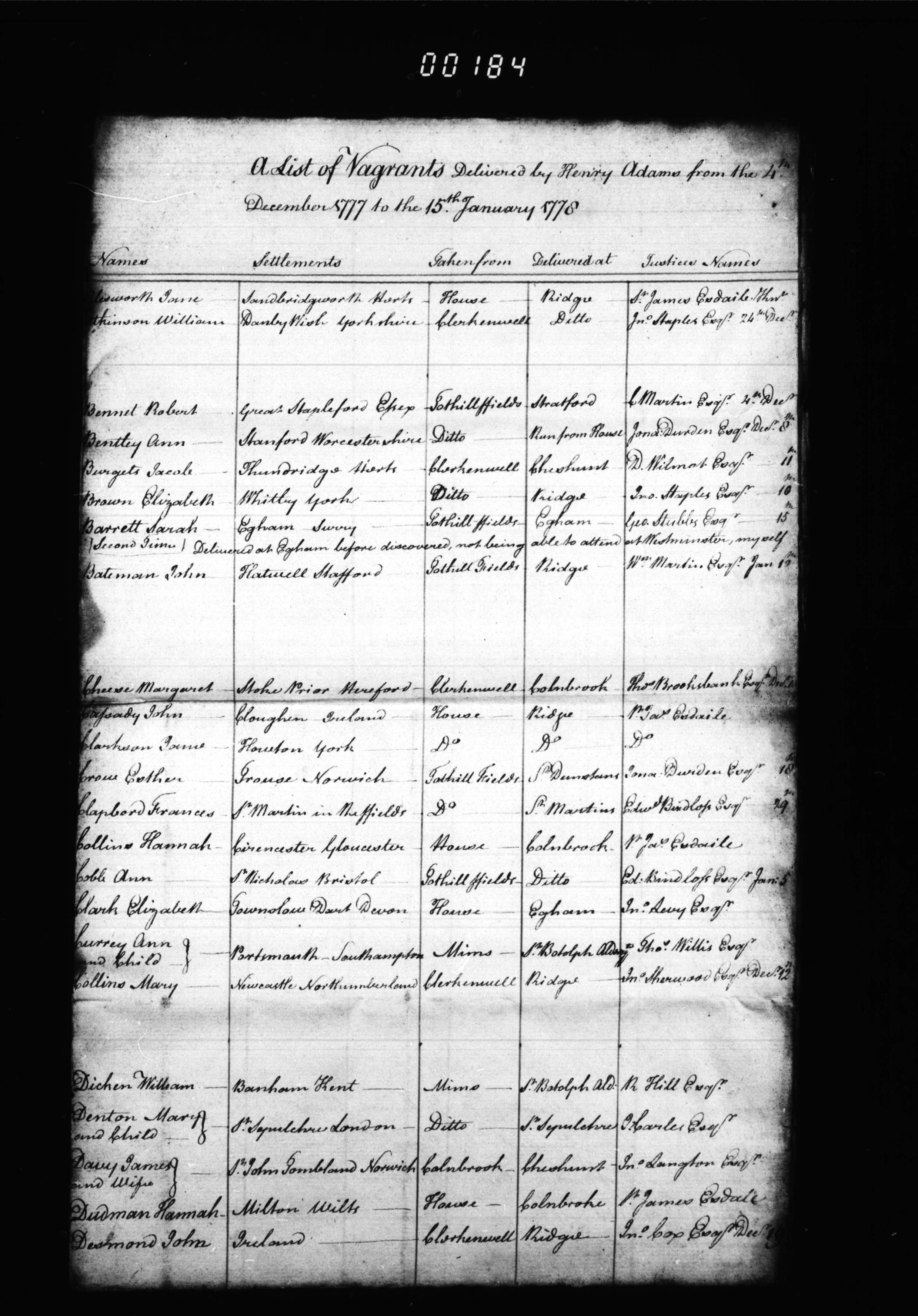
Figure 3: A sample list of vagrants expelled from Middlesex. ‘Middlesex Sessions Papers - Justices’ Working Documents’, (January 1778), London Lives, 1690-1800, LMSMPS50677PS506770118 (www.londonlives.org, version 2.0, 18 August 2018), London Metropolitan Archives.
As part of the “Vagrant Lives” project, the original vagrancy lists were converted into a scholarly dataset and published as:
- Adam Crymble, Louise Falcini, Tim Hitchcock, “Vagrant Lives: 14,789 Vagrants Processed by the County of Middlesex, 1777-1786”, Journal of Open Humanities Data, vol. 1, no. 1 (2015), http://doi.org/10.5334/johd.1.
Readers are invited to download and explore this published dataset and its documentation to understand the types of primary sources being modelled in this example.
Important Notes about the Dataset:
Gravity models will only return meaningful results if constructed for case studies that meet certain conditions. While it is not feasible to provide an exhaustive list, there were a few decisions the authors had to make when working with this dataset of vagrants, and they are worth repeating as a warning to readers who might be thinking about their own study.
-
These historical data in the “Vagrant Lives” dataset are not complete. 42 of a possible 65 such lists survive for the period 1777 to 1786, which represents approximately 75% of all vagrants expelled for whom there should be a record. The remaining primary sources are lost. It is important that the records one uses are either a complete or representative sample. The authors of the dataset believe the 75% of records that survived are representative of what we would find if we had all 100%. If this was not the case, modelling may not be appropriate.
-
The authors believe that migrants from all counties were equally likely to be arrested as vagrants, and that the total number of vagrants from a county is proportional to the amount of migration from that county. In other words, we do not believe that people from Cornwall, for example, were more likely to be arrested as vagrants than people from Leicestershire. Again, if this was not the case, modelling may not be appropriate.
-
The dataset contains details of vagrants from 32 of the 39 historic English counties (see Figure 4). The remaining 7 counties were not included in the analysis because of possibly incomplete data, and the reasons for this are cited in the original paper.2 If the missing counties had not been geographically clustered as they are, a gravity model might not have been appropriate.
-
The dataset contains very few “recidivists” - repeat offenders. Some migration channels in various points in history and places in the world include a great deal of seasonal, temporary, or repeat migration. If the migration you are attempting to model includes any of these, and you believe them to be distributed unevenly across your possible origin and destinations, a gravity model might not be appropriate.
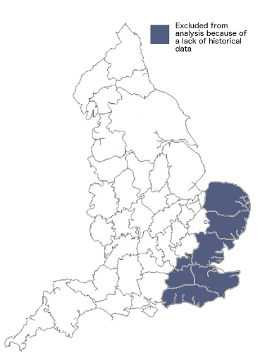
Figure 4: A map of historic English counties, showing counties excluded from the analysis
- A model of this sort should always contain moving entities that are of the same type as one another whenever possible (coffee beans and coffee beans, not coffee beans and bananas). Despite the fact that all of these individuals appear on the same types of lists, the “vagrants” in the sources represent three distinct types of people.
- The “vagabond poor” - the stereotypical poor individual from elsewhere.
- Demobilised soldiers who used the vagrancy system for a free ride home.
- Individuals expelled back to London from other counties (not relevant to the original research question and excluded here).
The first two groups represent migrants from elsewhere, but because they came to London via quite different paths - one as an economic migrants and one dumped on the docks after finishing work overseas - they were modelled separately in the original article. Splitting these two types of vagrants into two models meant more defensible results. Those were not the only two subsets we could have modelled, as any subset for which there was an intellectual case would also do (e.g. men and women).
For the sake of brevity, this tutorial will take readers through the modelling of the 3,262 “vagabond poor”, though the process for modelling the demobilised soldiers is exactly the same.
Preview of the Finished Model
The result of the modelling process can be seen in Figure 5. As you can see on the map, there are in fact regional anomalies. There is a cluster of counties in the West Midlands (four blue counties) that were over-sending migrants to London. There were also a number of counties in the centre of the map and towards the north that were under-sending migrants (red), and there are a few regional anomalies sprinkled around the country. The remainder of this tutorial will walk you through the process of making those types of discoveries from a set of historical data, starting with the mathematics that allow us to do this type of work.
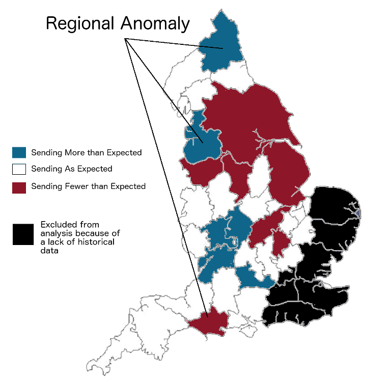
Figure 5: The anomalous counties in the original study, showing areas with fewer migrants than expected, more migrants than expected, and about the expected number.
The formula used to arrive at that result is provided below, with the following sections outlining the origins and rationale of that formula.
\[μ_{ij} = exp(β_{0} + β_{1}ln(P_{i}) + β_{2}ln(d_{ij}) + β_{3}Wh_{i} + β_{4}Wa_{i} + β_{5}WaT_{i})\]Regression Modelling, and the Mathematics Behind the Model
The example used in this tutorial is one of many “gravity models” or “spatial interaction models” that measure the way entities (often people) use spaces. They are part of what A.G. Wilson referred to as a “family of spatial interaction models”, and were developed from R.G. Ravenstein’s 1885 attempts to derive “laws” of migration that could explain or even predict the movement of populations, including an assertion that both distance and population are key factors in the flows of migration between two points 3. Wilson outlines many different equations (models), depending on what type of movement is under investigation and what information is known or unknown. For example, you would need to use a different or adapted model (equation) if your case study involved movement between multiple locations and multiple destinations. Gravity models are also the subject of active research, and scholars continue to refine their underlying mathematics as new ideas emerge. The formula used here is based upon the latest research to date, at the time the article was written. It is particularly indebted to earlier work by Tobler, Flowerdew, Aiken, Lovett, Abel, and Congdon, variously published between 1970 and 2010.4
From a mathematical perspective, our gravity model is a type of regression analysis, a means of comparing sets of variables in search of relationships between them. While not all gravity models use regression, the example in this tutorial does. This section covers in brief regression analyses, moving from a simple linear regression, to a multivariate linear regression, and finally to the negative binomial regression which is the basis of our model. Each builds upon the other.
- simple linear regression
- multivariate linear regression
- negative binomial regression (our gravity model)
Simple Linear Regression
The most basic regression analysis is a simple linear regression analysis. A simple linear regression of two variables (eg, county population, and number of vagrants) provides a way to quantify the relationship between those two variables. When you plot the values on a scatter plot (eg, county population on the x-axis, and number of vagrants on the y-axis), looking at the graph makes it clear that there is a loose but reasonably obvious linear relationship between them (Figure 6). Generally speaking, the greater the population, the more vagrants you find. The purpose of a simple linear regression is to calculate the formula that best represents the straight line that comes as close to as many of the points on the graph as possible. Since not all points fall directly on the line, but most are fairly close, Figure 6 suggests that population is a good, but not a perfect predictor of the number of vagrants from a given county.
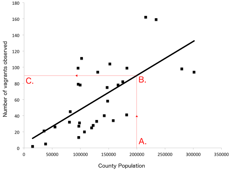
Figure 6: A simple linear regression of county population (x-axis) and number of vagrants observed, 1777-1786 (y-axis). To make this graph more readable, Yorkshire has been excluded because of its very large population.
There are many websites that provide calculator functions that will do this for you automatically, and proprietary software including Microsoft Excel and SPSS can also perform this calculation. The formula for a simple linear regression is:
\[y = α + βx\]- $y$ is a value on the y-axis (number of vagrants, in the example above).
- $α$ is the y-intercept. This is the value of $y$ when $x = 0$.
- $β$ is the slope of the regression line.
- $x$ is a value on the x-axis (the population of the county).
Many tutorials can teach you to conduct simple linear regressions.5 When you know $α$ and $β$, you can choose a value for either $x$ (population) or $y$ (number of vagrants), and then calculate the other. You can do that mathematically using the formula above, or you can eyeball it by looking at the graph in Figure 6 if you only need a rough measure. If you want to know the estimated number of vagrants for a county with a population of 200,000 ($A.$ on Figure 6), then you find where $x$ and $y$ meet ($B.$), and finally the y-intercept for that value ($C.$). In other words: if population is 200,000, how many vagrants would we expect? According to the graph, about 90.
Multivariate Linear Regression
A multivariate linear regression (multiple variable) is a more powerful version of the above. Instead of handling two variables ($y$ and $x$), it can handle an unlimited number. The principles are exactly the same as the simple linear regression above. Again, there are online calculators that can conduct a multivariate linear regression, or we can calculate it using the following equation:
\[y = β_{0} + β_{1}(x_{1}) + β_{2}(x_{2}) + ... + β_{p}(x_{p})\]The formula works the same way, and the symbols mean exactly the same as above, with the exception of $β_{0}$ and $p$.
- $β_{0}$ is the y-intercept in a multivariate linear regression (represented as $α$ in the Simple Linear Regression formula). From our perspective, it is the same.
- $p$ simply stands for “the last/final variable” and is used to show that there is no upper limit to the number of possible variables.
Unlike in the simple linear regression formula, in this example, there are multiple variables, each of which has a line of best fit, each of which has a slope of the line that has to be calculated ($β_{1}$, $β_{2}$, etc). It is difficult to draw a multivariate linear regression on a scatterplot because you would need a new dimension for each added variable. In principle it is the same as the simpler version, but with more axes.
You can add and remove the number of variables to suit your own needs. Keeping in mind that $y$ counts as one of the variables (vagrants observed, in this case), a three, four, and five variable version of the above equation looks like this:
Three Variable ($y$ Plus 2 Independent Variables):
\[y = β_{0} + (β_{1}x_{1}) + (β_{2}x_{2})\]Four Variable ($y$ Plus 3 Independent Variables):
\[y = β_{0} + (β_{1}x_{1}) + (β_{2}x_{2}) + (β_{3}x_{3})\]Five Variable ($y$ Plus 4 Independent Variables):
\[y = β_{0} + (β_{1}x_{1}) + (β_{2}x_{2}) + (β_{3}x_{3}) + (β_{4}x_{4})\]This is not quite our model yet. However, the model we will use is very like this and includes five independent variables plus the number of observed vagrants for each county, described below in detail. For our model, taking a multivariate approach to regression allows us to ask much more complex questions, such as, how many vagrants would we expect if:
- if population is 200,000
- distance from London is 55km
- average wages are 80 shillings per month
- and they have risen by 12% in recent years
- while the local price of wheat is 65 shillings per bushel?
If this imaginary county existed, the answer is: about 206 vagrants. That’s very different than the 90 estimated by the simple linear regression, suggesting other factors apart from population had a big influence on the distribution. The next section will explain how we know that 206 is the most likely value for this imaginary county.
Negative Binomial Regression
The formula used in our gravity model is extremely similar to the one above. It uses a negative binomial regression model,6 which is a multivariate regression model with some tweaks. These tweaks are necessary because the nature of our sample data is most likely to follow a Negative Binomial Distribution.
In probability statistics, there are a number of different probability distributions. These are often represented visually as a curve, which shows the likelihood of each possible outcome in a given test. These curves vary widely - some are long and low, others have a sharp peak in the middle and very short tails, while others still take on more interesting patterns. Statisticians have come to recognise that certain types of tests using certain types of data are more likely to follow certain probability distributions. Knowing this means that statisticians have been able to tweak formulas to different types of probability tests, to return the most likely outcome. As historians we can use their findings to apply the best possible model to our historical data.
As it happens, our vagrants are best suited to a negative binomial distribution. The reasons for this are that they represent count data (1, 2, 53 vagrants) that must be whole numbers (no 0.5 vagrants) and cannot be negative (no -9 vagrants). Earlier gravity modelling conducted in the 1980s tended to use a Poisson Distribution for modelling human migration. The best approach for gravity models is still a point of academic debate, with some scholars opting for a Negative Binomial approach, and others sticking with the Poisson distribution.7 It is possible that another probability distribution entirely is most appropriate for your own data. If you were modelling trade surpluses or deficits (which could be + or -), your data may not follow a negative binomial distribution, and the author recommends speaking to a statistician about the most appropriate option.
What this means for us in this example is that the formula changes slightly. In particular, we no longer solve for $y$, but for the natural logarithm ($ln$) of the population mean ($μ$). You can read more about this type of formula in Michael L. Zwilling’s work8.
Multivariate Regression Model:
\[y = ...\]Negative Binomial Regression Model:
\[ln(μ) = ...\]The full formula looks like this:
\[ln(μ) = β_{0} + (β_{1}x_{1}) + (β_{2}x_{2}) + (β_{3}x_{3}) + (β_{4}x_{4}) + (β_{5}x_{5})\]To make it easier to solve, we can rewrite this formula to isolate $μ$ on the left side of the equation by counteracting the natural log ($ln$) - effectively removing it from the calculation. To do so, we must perform the inverse of natural log on both sides of the equation. The inverse of a natural log ($ln$) is the exponential function ($exp$). This means multiplying natural log by the exponential function on the left side of the equation (resulting in 1, and making it redundant since 1($μ$) is $μ$). You must also do the same on the right side.
This means everything on the right side of the new equation must be multiplied by $exp()$:
\[μ = exp(β_{0} + (β_{1}x_{1}) + (β_{2}x_{2}) + (β_{3}x_{3}) + (β_{4}x_{4}) + (β_{5}x_{5}))\]The above is the basis of the equation used in the Economic History Review article upon which this tutorial is based, and should be the starting point for your own studies if you are modelling data that follows a negative binomial distribution. You may notice this is slightly different than the model used in the original article, which is seen below and explained in the next section. The differences are largely superficial and tailored to the very specific case study.9
The Final Gravity Model:
\[μ_{ij} = exp(β_{0} + (β_{1}ln(P_{i}) + (β_{2}ln(d_{ij}) + (β_{3}Wh_{i}) + (β_{4}Wa_{i}) + (β_{5})WaT_{i}))\]$μ_{ij}$ stands for the population interaction between origin $i$ and destination $j$ - in this case, the number of vagrants moving to London from that area. The remaining symbols represent each of the five variables used in the example case study, and will be explained more fully below.
The Three Steps of Gravity Modelling
To make this method as accessible as possible, we will take a step-by-step approach to understand the components of the formula and how to calculate it for the example data, which we will begin to compile in the next step.
In order to determine the most likely distribution of migrants across the 32 counties, the modelling process involves three steps:
- Deciding on variables and gathering the relevant data.
- Determining the relative importance (weighting) of each variable.
- Applying the weightings for each county to get a predicted number of movements.
Each of those three steps will involve finding certain parts of the equation so that we can ultimately solve it mathematically. This three-step process provides a numerical estimate of migrants (or coffee beans/widgets) for each territory in the model, allowing for a final step: historical interpretation.
Step 1 - Deciding on Variables and Gathering the Relevant Data
The first step is to decide which independent variables / influencing factors to include in the model. These are the variables that we think will influence the distribution of our migrants. How many variables you choose to include and what they are is part art, part science, and part luck.
It is art because you understand your data better than anyone, so should have an idea of the factors that might be most important. It is science because for most types of migration or trade, other scholars have already published about push or pull factors that are known to influence those types of distributions.10 And luck because in order to use a given factor, you need to have reliable historical data for each and every territory in your model. If those data do not exist, or the records do not allow you to create a complete set for a given variable, you are unable to include it.
Influencing factors need to be considered on a case by case basis and to draw on your subject specialist expertise. There is not a right answer when it comes to the number or types of variables to use, but it is a good idea not to try to over-model with a long list. A few very relevant factors is probably better than many weak markers.
There are also a number of wrong ways you can include variables. A gravity model will not work unless each variable meets the following criteria:
- Numerical
- Complete
- Reliable
Numerical Data Only
As the gravity model is a mathematical equation, all input variables must be numerical. That could be a count (population), spatial measure (area, distance, etc), time (hours from London on foot), percentage (wage increase/decrease), currency value (wages in shillings), or some other measure of the places involved in the model.
Numbers must be meaningful and cannot be nominal categorical variables which act as a stand-in for a qualitative attribute. For example you cannot arbitrarily assign a number and use it in the model if the number doesn’t have meaning (eg, road quality = good, or road quality = 4). Though the latter is numerical it is not a measure of road quality. Instead, you might use the average travel speed in miles per hour as a proxy for road quality. Whether average speed is a meaningful measure of road quality is up to you to determine and defend as the author of the study.
Generally speaking, if you can measure it or count it, you can model it.
Complete Data Only
All categories of data must exist for each point of interest. That means that all of the 32 counties under analysis must have reliable data for each push and pull factor. You cannot have any gaps or blanks, such as one county where you don’t have the average wage.
Reliable Data Only
The computer science adage “garbage in, garbage out” also applies to gravity models, which are only as reliable as the data used to build them. Beyond choosing robust and reliable historical data from sources you can trust, there are lots of ways to make mistakes that will render the outputs of your model meaningless. For example, it is worth making sure that the data you have exactly match the territories (eg, county data to represent counties, not city data to represent a county).
Depending on the time and place of your study, you may find it difficult to obtain a reliable set of data upon which to base your model. The further back in the past one’s study, the more difficult that may be. Likewise, it may be easier to conduct these types of analyses in societies that were heavily bureaucratic and left a good surviving paper trail, such as in Europe or North America.
To ensure data quality in this case study, each variable was either reliably calculated or derived from published peer-reviewed historical data (see Table 1). Exactly how these data were compiled can be read in the original article where it was explained in depth.11
Our Five Model Variables
With the above principles in mind, we could have chosen any number of variables, given what we knew about migration push and pull factors. We settled on five (5), chosen based on what we thought would be most important, and which we knew could be backed up with reliable data.
| Variable | Source |
|---|---|
| population at origin | 1771 values, Wrigley, “English county populations”, pp. 54-5.12 |
| distance from London | calculated with software |
| price of wheat | Cannon and Brunt, “Weekly British Grain Prices”13 |
| average wages at origin | Hunt, “Industrialization and Regional Inequality”, pp. 965-6.14 |
| trajectory of wages | Hunt, “Industrialization and Regional Inequality”, pp. 965-6.15 |
Table 1: The five variables used in the model, and the source of each in the peer reviewed literature
Having decided on these variables, the co-author of the original study, Adam Dennett, decided to rewrite the formula to make it self-documenting so that it was easy to tell which bits pertained to each of these five variables. This is why the formula shown above looks different than the one in the original research paper. The new symbols can be seen in Table 2:
| Symbol | Meaning |
|---|---|
| $i$ | the county of origin |
| $j$ | London (destination) |
| $P$ | Population at origin ($i$) |
| $d$ | Distance from origin ($i$) to London ($j$) |
| $Wh$ | Price of Wheat at origin ($i$) |
| $Wa$ | Average wages at origin ($i$) |
| $WaT$ | Wage trajectory at origin ($i$) |
Two additional variables $i$ and $j$, mean “at point of origin” and “at London” respectively. $Wa_{i}$ means “wage levels at the point of origin” whereas $Wa_{j}$ would mean “wage levels in London”. These seven new symbols can replace the more generic ones in the formula:
\[μ_{ij} = exp(β_{0} + (β_{1}P_{i}) + (β_{2}d_{ij}) + (β_{3}Wh_{i}) + (β_{4}Wa_{i}) + (β_{5}WaT_{i}))\]This is now more verbose and a slightly self-documented version of the previous equation. Both solve mathematically in exactly the same way, as the changes are purely superficial and for the benefit of a human user.
The Completed Variable Dataset
To make the tutorial quicker easier to complete, the data for each of the 5 variables and each of the 32 counties have already been compiled and cleaned, and can be seen in Table 3 or downloaded as a csv file. This table also includes the known number of vagrants from that county, as observed in the primary source record:
| County | Vagrants | $d$ km to London | $P$ Population (persons) | $Wa$ Average Wage (shillings) | $WaT$ Wage Trajectory 1767-95 (% change) | $Wh$ Wheat Price (shillings) |
|---|---|---|---|---|---|---|
| Bedfordshire | 26 | 61.9 | 54836 | 87 | 1.149 | 61.79 |
| Berkshire | 111 | 61.7 | 101939 | 90 | 4.44 | 63.07 |
| Buckinghamshire | 79 | 46.7 | 95936 | 96 | -8.33 | 63.09 |
| Cambridgeshire | 32 | 86.8 | 80497 | 88 | 11.36 | 60.05 |
| Cheshire | 34 | 255.1 | 158038 | 80 | 35.00 | 69.19 |
| Cornwall | 40 | 364.6 | 142179 | 81 | 14.81 | 67.94 |
| Cumberland | 13 | 407.3 | 96862 | 78 | 38.46 | 64.42 |
| Derbyshire | 28 | 196.9 | 122593 | 75 | 48.00 | 68.02 |
| Devon | 98 | 272.5 | 279652 | 89 | -7.87 | 69.98 |
| Dorset | 27 | 176.8 | 97262 | 81 | 22.22 | 67.30 |
| Durham | 25 | 380.7 | 119779 | 78 | 33.33 | 63.16 |
| Gloucestershire | 162 | 157.1 | 215576 | 81 | 9.88 | 66.54 |
| Hampshire | 78 | 102.4 | 166648 | 96 | 6.25 | 61.45 |
| Herefordshire | 45 | 190.5 | 81882 | 70 | 28.57 | 62.05 |
| Hertfordshire | 99 | 35.3 | 95868 | 90 | 4.44 | 63.82 |
| Huntingdonshire | 21 | 87.5 | 35370 | 89 | 7.87 | 58.72 |
| Lancashire | 94 | 281.8 | 301407 | 78 | 55.13 | 71.65 |
| Leicestershire | 20 | 146.1 | 107028 | 79 | 65.82 | 64.84 |
| Lincolnshire | 41 | 179.8 | 181814 | 84 | 26.19 | 58.73 |
| Northamptonshire | 33 | 107.6 | 128798 | 78 | 21.79 | 63.81 |
| Northumberland | 58 | 440.0 | 148148 | 72 | 70.83 | 58.22 |
| Nottinghamshire | 31 | 187.5 | 98216 | 108 | 0.00 | 61.30 |
| Oxfordshire | 78 | 86.8 | 99354 | 84 | 25.00 | 64.23 |
| Rutland | 2 | 132.5 | 15123 | 90 | 10.00 | 64.12 |
| Shropshire | 75 | 214.0 | 147303 | 76 | 18.42 | 66.50 |
| Somerset | 159 | 180.4 | 234179 | 77 | 3.90 | 68.29 |
| Staffordshire | 82 | 185.3 | 175075 | 76 | 18.42 | 67.80 |
| Warwickshire | 104 | 149.3 | 152050 | 96 | -3.13 | 65.05 |
| Westmorland | 5 | 365.0 | 38342 | 74 | 62.16 | 71.05 |
| Wiltshire | 99 | 131.7 | 182421 | 84 | 20.24 | 63.64 |
| Worcestershire | 94 | 164.4 | 130757 | 81 | 25.93 | 65.78 |
| Yorkshire | 127 | 282.2 | 651709 | 80 | 58.33 | 61.87 |
The final difference between this formula and the one used in the original article, is that two of the variables happen to have a stronger relationship with vagrancy when plotted naturally logarithmically. They are population at origin ($P$) and distance from origin to London ($d$). What this means is that for the data in this study, the regression line (sometimes called line of best fit) is a better fit when the data has been logged than when it has not been. You can see this in Figure 7, with the non-logged population figures on the left, and the logged version on the right. More of the points are closer to the line of best fit on the logged graph than on the non-logged one.
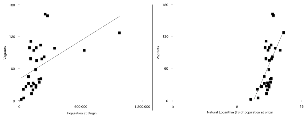
Figure 7: Number of Vagrants plotted against population at origin (left), and natural log of population of origin (right) with a simple regression line overlayed on both. Note the stronger relationship between the two variables visible on the second graph.
Because this is the case with this particular data (your own data in a similar type of study may not follow this pattern), the formula was adjusted to use the naturally logged versions of these two variables, resulting in the final formula used in the gravity model (Figure 8). We could not possibly have known about the need for this adjustment until after we had collected our variable data:

Figure 8: The final gravity model formula broken down by steps and colour-coded. Elements in black are mathematical operations. Elements in Blue represent our variables, which we have just gathered (Step 1). Elements in Red represent the weightings of each variable, which we must calculate (Step 2), and the Element in Orange is the final estimate of vagrants from that county, which we can calculate once we have the other information (Step 3).
The values in Table 3 give us everything we need to fill in the Blue parts of each equation in Figure 8. We can now turn our attention to the Red parts, which tell us how important each variable is in the model overall, and gives us the numbers we need to complete the equation.
Step 2: Determining the Weightings
The weightings for each variable tell us how important that push/pull factor is relative to the other variables when trying to estimate the number of vagrants that should have come from a given county. The $β$ parameters must be determined across the whole data set from the known data. With these to hand we will be able to compare individual origin-specific observations with the general model. We can then examine these and identify over and under predicted flows between the various origins and the destination.
At this stage we do not know how important each is. Perhaps wheat price is a better predictor of migration than distance? We will not know until we calculate the values of $β1$ through $β5$ (the weightings) by solving the equation above. The y-intercept ($β0$) only possible to calculate once you know all of the others ($β1-β5$). These are the RED values in Figure 8 above. The weightings can be seen in Table 4 and in Table A1 of the original paper.16 We will now demonstrate how we came to these values.
| Variable | Weighting | Symbol |
|---|---|---|
| y-intercept | -3.84678 | $β0$ |
| population | 1.235208 | $β1$ |
| distance | -0.541863 | $β2$ |
| wheat price | -0.023957 | $β3$ |
| wages | -0.025184 | $β4$ |
| wage trajectory | -0.013779 | $β5$ |
To calculate these values long-hand requires an incredible amount of work. We will use a quick solution in the R programming language that takes advantage of William Venables and Brian Ripley’s MASS package that can solve negative binomial regression equations like our gravity model with a single line of code. However, it is important to understand the principles behind what one is doing in order to appreciate what the code does (note the following sections do not DO the calculation, but explain its steps for you; we will do the calculation with the code further down the page).
Calculating the Individual Weightings (in Principle)
$β_{1}$, $β_{2}$, etc, are the same as $β$ in the Simple Linear Regression model above, which is the slope of the regression line (the rise over the run, or how much $y$ increases when $x$ increases by 1). The only difference here between a Simple Linear Regression and our gravity model is that we have to calculate 5 slopes instead of 1.
A Simple Linear Regression \(y = α + βx\)
We will need to solve for each of these five slopes before we can calculate the y-intercept in the next step. That is because the slopes of the various $β$ values are part of the equation for calculating the y-intercept.
The formula for calculating $β$ in a regression analysis is:
\[β = r (\frac{s_{y}}{s_{x}})\]- We already know that $β$ is the slope, which is what we are trying to calculate.
- $r$ is Pearson’s correlation coefficient, which we are going to compute
- $s_{y}$ is the standard deviation of $y$
- $s_{x}$ is the standard deviation of $x$
Pearson’s Correlation Coefficient
Pearson’s correlation coefficient can be calculated long-hand but it’s a rather long calculation in this case, requiring 64 numbers. There are some great video tutorials in English available online if you would like to see a walk-through of how to do the calculations long-hand.17 There are also a number of online calculators that will calculate $r$ for you if you provide the data. Given the large number of digits to compute, I would recommend a website with a built in tool designed to make this calculation. Make sure you choose a reputable site, such as one offered by a university.
Calculating $s_{y}$ & $s_{x}$ (Standard Deviation)
Standard deviation is a way of expressing how much variation from the mean (average) there is in the data. In other words, is the data fairly clustered around the mean, or is the spread much wider?
Again, there are online calculators and statistical software packages that can do this calculation for you if you provide the data.
With the above values, you can calculate $β_{1}$. This will have to be done once for each of the five variables $β_{1}$ to $β_{5}$. These values allow you to calculate the y-intercept, $β_{0}$
Calculating $β_{0}$ (the y-Intercept)
Next, we have to calculate the y-intercept. The formula for calculating the y-intercept in a Simple Linear Regression is:
\[β_{0} = \bar{y} - β \times \bar{x}\]However, the calculation becomes much more complicated in a multiple regression analysis, as each variable influences the calculation. This makes doing it by hand very difficult, and is one of the reasons we opt for a programmatic solution.
The Code for Calculating the Weightings
The MASS statistical package, written for the R programming language, has a function that can solve negative binomial regression equations, making it very easy to calculate what would otherwise be a very difficult long-hand formula.
This section assumes you have installed R and have installed the MASS package. If you have not done so you will have to before proceeding. Taryn Dewar’s tutorial on R Basics with Tabular Data includes R installation instructions.
To use this code, you will need to download a copy of the dataset of the five variables plus the number of observed vagrants from each of the 32 counties. This is available above as Table 3, or can be downloaded as a .csv file. Whatever mode you choose, save the file as VagrantsExampleData.csv. If you are using a Mac make sure you save it as a Windows format .csv file. Open VagrantsExampleData.csv and familiarise yourself with its contents. You should notice each of the 32 counties, along with each of the variables we’ve discussed throughout this tutorial. We will be using the column headers to access this data with our computer programme. I could have called them anything, but in this file they are:
vagrantspopulationdistancewheatwageswageTrajectory
In the same directory as you saved the csv file, create and save a new R script file (you can do this with any text editor or with RStudio, but do not use a word processor like MS Word). Save it as weightingsCalculations.r.
We will now write a short programme that:
- Installs the MASS package
- Calls the MASS package so we can use it in our code
- Stores the contents of the .csv file to a variable that we can use programmatically
- Solves the gravity model equation using the dataset
- Outputs the results of the calculation.
Each of these tasks will be achieved in turn with a single line of code
install.packages("MASS")
library(MASS)


gravityModelData <- read.csv("VagrantsExampleData.csv")

gravityModel <- glm.nb(vagrants~log(population)+log(distance)+wheat+wages+wageTrajectory, data=gravityModelData)
summary(gravityModel)
Copy the above code into your weightingsCalculations.r file and save. You can now run the code using your favourite R environment (I use RStudio) and the results of the calculation should appear in the console window (what this looks like will depend upon your environment). You may need to set the Working Directory of your R environment to the directory containing your .csv and .r files. If you are using RStudio you can do this via the menus (Session -> Set Working Directory -> Choose Directory). You can also achieve the same with the command:
setwd(PATH) #change "PATH" to the full location on your computer where the files can be found
Notice that line 4 is the line that solves the equation for us, using the glm.nb function, which is short for “generalized linear model - negative binomial”. This line requires a number of inputs:
- our variables using the column headers as written in the .csv file, along with any logging that must be done to them (
vagrants, log(population), log(distance),wheat,wages,wageTrajectory). If you were running a model with your own data, you would adjust these to reflect your column headers in your dataset. - where the code can find the data - in this case a variable we’ve defined in line 3 called
gravityModelData.
The outputs of the calculation can be seen in Figure 9:
.](/images/gravity-model/figure9.png)
Figure 9: The summary of the above code, showing the weightings for each variable and the y-intercept, listed under the ‘Estimate’ heading ($\beta_{0}$ to $\beta_{5}$. This summary also shows a number of other calculations, including statistical significance.
Step 3: Calculating the Estimates for Each County
Because we now have the y-intercept ($β0$), the weightings ($β1-5$), and the 5 variable values for each county ($P$, $d$, $Wh$, $Wa$, $WaT$), we have all the numbers we need to solve for the model’s predicted value for a county: the final result.
We have to do this once for each of the 32 counties.
You could do this with a scientific calculator, by creating a spreadsheet formula, or writing a computer programme. To do this automatically in R, you can add the following to your code and re-run the programme. This for loop calculates the expected number of vagrants from each of the 32 counties in the example and prints the results for you to see:
for (entry in c(gravityModelData$County)){
  print(paste("Result for County ", gravityModelData$County[entry],
              (exp(-3.848
                  + (1.235 * log(gravityModelData$population[entry]))
                  + (-0.542 * log(gravityModelData$distance[entry]))
                  + (-0.024 * gravityModelData$wheat[entry])
                  + (-0.025 * gravityModelData$wages[entry])
                  + (-0.014 * gravityModelData$wageTrajectory[entry])
              ))
        ))
}
To build understanding, I suggest doing one county long-hand. This tutorial will use Hertfordshire as the long-hand example (but the process is exactly the same for the other 31 counties).
Using the data for Hertfordshire in Table 3, and the weightings for each variable in Table 4, we can now complete our formula, which will give the result of 95:
estimated vagrants =
  exp(y-intercept
  + (#population calculation)
  + (#distance calculation)
  + (#wheat price calculation)
  + (#wages calculation)
  + (#wage trajectory calculation)
  )
First, let’s swap out the symbols for the numbers, taken from the tables mentioned above.
estimated vagrants =
  exp(-3.848  						#y-intercept
  + (1.235 * ln(97389)) 			#population calculation
  + (-0.542 * ln(35.3)) 	#distance calculation
  + (-0.024 * 63.82) 			#wheat price calculation
  + (-0.025 * 90) 					#wages calculation
  + (-0.014 * 4.44)			#wage trajectory calculation
  )
Then, start to calculate values to get to the estimate. Remembering mathematical order of operations, multiply values before adding. So start by calculating each variable (you can use a scientific calculator for this):
estimated vagrants =
  exp(-3.848  						#y-intercept
  + (14.185788655431) 				#population calculation
  + (−1.93162456646) 				#distance calculation
  + (−1.53168) 				#wheat price calculation
  + (-2.25) 							#wages calculation
  + (−0.06216)				#wage trajectory calculation
  )
The next step is to add the numbers together:
estimated vagrants = exp(4.56232408897)
And finally, to calculate the exponential function (use a scientific calculator):
estimated vagrants = 95.8059926832
We have dropped the remainder and declared that the estimated number of vagrants from Hertfordshire in this model is 95. You have to conduct the same calculations for each of the other counties, which you could speed up by using a spreadsheet program. Just to make sure you can do it again, I’ve also included the numbers for Buckinghamshire:
Hertfordshire
\[95 = estimated vagrants = exp(-3.848 + (1.235 * ln(97389)) + (-0.542 * ln (35.3)) + (-0.024 * 63.82) + (-0.025 * 90) + (-0.014 * 4.44) )\]Buckinghamshire
\[83 = estimated vagrants = exp(-3.848 + (1.235 * ln(95936)) + (-0.542 * ln (46.7)) + (-0.024 * 63) + (-0.025 * 96) + (-0.014 * -8.33) )\]I recommend choosing one other county and calculating it long-hand before moving on, to make sure you can do the calculations on your own. The correct answer is available in Table 5, which compares the observed values (as seen in the primary source record) to the estimated values (as calculated by our gravity model). The “Residual” is the difference between the two, with a large difference suggesting an unexpected number of vagrants that might be worth a closer look with one’s historian’s hat on.
| County | Observed Value | Estimated Value | Residual |
|---|---|---|---|
| Bedfordshire | 26 | 41 | -15 |
| Berkshire | 111 | 76 | 35 |
| Buckinghamshire | 79 | 83 | -4 |
| Cambridgeshire | 32 | 48 | -16 |
| Cheshire | 34 | 44 | -10 |
| Cornwall | 40 | 42 | -2 |
| Cumberland | 13 | 21 | -8 |
| Derbyshire | 28 | 36 | -8 |
| Devon | 98 | 121 | -23 |
| Dorset | 27 | 36 | -9 |
| Durham | 25 | 31 | -6 |
| Gloucestershire | 162 | 123 | 39 |
| Hampshire | 78 | 92 | -14 |
| Herefordshire | 45 | 39 | 6 |
| Hertfordshire | 99 | 95 | 4 |
| Huntingdonshire | 21 | 18 | 3 |
| Lancashire | 94 | 84 | 10 |
| Leicestershire | 20 | 28 | -8 |
| Lincolnshire | 41 | 86 | -45 |
| Northamptonshire | 33 | 78 | -45 |
| Northumberland | 58 | 29 | 29 |
| Nottinghamshire | 31 | 28 | 3 |
| Oxfordshire | 78 | 52 | 26 |
| Rutland | 2 | 4 | -2 |
| Shropshire | 75 | 66 | 9 |
| Somerset | 159 | 145 | 14 |
| Staffordshire | 82 | 85 | -3 |
| Warwickshire | 104 | 70 | 34 |
| Westmorland | 5 | 5 | 0 |
| Wiltshire | 99 | 95 | 4 |
| Worcestershire | 94 | 53 | 41 |
| Yorkshire | 127 | 207 | -80 |
Step 4 - Historical Interpretation
At this stage, the modelling process is complete and the final stage is historical interpretation.
The original published article upon which this case study was based, is devoted primarily to interpreting what the results of the modelling mean to our understanding of lower class migration in the eighteenth century. As seen in the map in Figure 5, there were parts of the country that the model strongly suggested were either over- or under-sending lower class migrants to London.
The co-authors offered their interpretations as to why those patterns may have appeared. These interpretations varied by place. In areas of the North of England that were rapidly industrialising, such as Yorkshire or Manchester, the opportunities locally appeared to give people fewer reasons to leave, resulting in lower than expected migration to London. In declining areas to the west, such as Bristol, the lure of London was stronger as more people left seeking work in the capital.
Not all of the patterns were expected. Northumberland in the far north east proved to be a regional anomaly, sending far more (female) migrants to London than we would expect to see. Without the outputs of the model, it is unlikely that we would have thought to consider Northumberland at all, particularly because it was so far from the Metropolis and we presumed would have weak ties to London. The model thus provided new evidence for us to consider as historians and changed our understanding of the London-Northumberland relationship. A full discussion of our findings can be read in the original article.18
Taking Your Knowledge Forward
After having tried this example problem, you should have a clear understanding of how to use this example formula, as well as whether or not a gravity model might be an appropriate solution for your research problem. You have the experience and vocabulary to approach and discuss gravity models with an appropriately mathematically literate collaborator should you need to, who can help you to adapt it to your own case study.
If you are fortunate enough to also have data about migrants moving to late eighteenth century London and you want to model it using the same five variables listed above, this formula would work as-is - there’s an easy study here for someone with the right data. However, this model does not only work for studies about migrants moving to London. The variables can change, and the destination does not need to be London. It would be possible to use a gravity model to study migration to ancient Rome, or twenty-first century Bangkok, if you have the data and the research question. It does not even need to be a model of migration. To use the Colombian coffee case study from the introduction, which focuses on trade rather than migration, Table 6 shows a viable use of the same formula, unaltered.
| Criteria | Coffee Exporting Example |
|---|---|
| ONE point of origin | coffee exports from the port of Barranquilla, Colombia |
| MULTIPLE finite destinations | the 21 countries of the Western Hemisphere in 1950 |
| FIVE explanatory variables | (1) number of Atlantic Ocean ports in receiving country (2) miles from Colombia, (3) Gross Domestic Product of receiving country, (4) Domestic Coffee grown in tons, (5) coffee shops per 10,000 people |
There is a long history of gravity models in academic scholarship. To use one effectively for research, you need to understand the basic theory and mathematics behind them and the reasons that they have developed as they have. It is also important to understand their limits and conditions for using them properly, some of which were discussed above. It might also help to know:
-
A gravity model like the one used in this example can only work in an enclosed system. The above model had only 32 possible points of origin, making it possible to run the model 32 times. An unknown or infinitely large number of points of origin (or destinations depending on your model), would require a different equation.
-
The gravity model concept is also built on the premise that movements (migration, trade, etc) are based on a collection of voluntary individual decisions that might be influenced by outside factors, but are not wholly controlled by them. For example, voluntary migrations or purchases made of free will could be modelled using this technique, but forced migration, compulsory purchase, or natural processes such as bird migration or river flow may not follow the same principles and therefore a different type of model may be needed.
-
Gravity models can be used to predict the behaviour of populations but not individuals, and therefore attempts to model data should include a large number of movements to ensure statistical significance.
There are many more pitfalls, but also tremendous possibilities. It is my hope that this walk-through of a gravity model, and its accompanying published research, will make this powerful tool more accessible for historians. If you are planning to use a gravity model in your scholarly research, the author strongly recommends the following articles:
- Wilson, A. G., ‘A family of spatial interaction models, and associated developments’, Environment and Planning A, 3 (1971), pp. 1–32.
- Flowerdew, R. and Aitkin, M., ‘A method of fitting the gravity model based on the Poisson distribution’, Journal of Regional Science, 22 (1982), pp. 191–202.
- Flowerdew, R. and Lovett, A., ‘Fitting constrained Poisson regression models to interurban migration flows’, Geographical Analysis, 20 (1988), pp. 297–307.
- Congdon, P., ‘Approaches to modelling overdispersion in the analysis of migration’, Environment and Planning A, 25 (1993), pp. 1481–510.
- Flowerdew, R., ‘Modelling migration with Poisson regression’, in J. Stillwell, O. Duke-Williams, and A. Dennett, eds., Technologies for migration and commuting analysis: spatial interaction data applications (Hershey, Pa., 2010), pp. 261–79.
- Abel, G. J., ‘Estimation of international migration flow tables in Europe: international migration flow tables’, Journal of the Royal Statistical Society, Series A (Statistics in Society), 173 (2010), pp. 797–825.
Acknowledgements
With thanks to Angela Kedgley, Sarah Lloyd, Tim Hitchcock, Joe Cozens, Katrina Navickas, and Leanne Calvert for reading and commenting on earlier drafts of this article. Also thanks to the British Academy for funding the writing workshop in Bogotá, Colombia at which this article was drafted. And finally to Adam Dennett for introducing me to these wonderful formulae and unleashing their potential for historians.
Endnotes
-
For a deeper understanding of vagrancy see Hitchcock, Tim, Adam Crymble, and Louise Falcini, “Loose, Idle, and Disorderly: Vagrancy Removal in Late Eighteenth Century Middlesex”, Social History, vol. 39, no. 4 (2014), 509-527. ↩
-
Crymble, A, A. Dennett, and T. Hitchcock, “Modelling regional imbalances in English plebeian migration to late eighteenth-century London”, Economic History Review, vol. 71, no. 3 (2018), 751. ↩
-
Ravenstein, R.G., ‘The Laws of Migration’, Journal of the Statistical Society of London, 48 (1885), 167-235; Wilson, A. G., ‘A family of spatial interaction models, and associated developments’, Environment and Planning A, 3 (1971), pp. 1–32. ↩
-
Tobler, W.R., ‘A Computer Movie Simulating Urban Growth in the Detroit Region’, Economic Geography, 46 (1970), 234-240; Flowerdew, R. and Aitkin, M., ‘A method of fitting the gravity model based on the Poisson distribution’, Journal of Regional Science, 22 (1982), pp. 191–202; Flowerdew, R. and Lovett, A., ‘Fitting constrained Poisson regression models to interurban migration flows’, Geographical Analysis, 20 (1988), pp. 297–307; Congdon, P., ‘Approaches to modeling overdispersion in the analysis of migration’, Environment and Planning A, 25 (1993), pp. 1481–510; Flowerdew, R., ‘Modelling migration with Poisson regression’, in J. Stillwell, O. Duke-Williams, and A. Dennett, eds., Technologies for migration and commuting analysis: spatial interaction data applications (Hershey, Pa., 2010), pp. 261–79; Abel, G. J., ‘Estimation of international migration flow tables in Europe: international migration flow tables’, Journal of the Royal Statistical Society, Series A (Statistics in Society), 173 (2010), pp. 797–825. ↩
-
For English speakers, the author recommends Eugene O’Loughlin, ‘How To…Perform Simple Linear Regression by Hand’, YouTube (23 December 2015): https://www.youtube.com/watch?v=GhrxgbQnEEU. ↩
-
“Chapter 326: Negative Binomial Regression”, NCSS Stats Software (n.d.): https://ncss-wpengine.netdna-ssl.com/wp-content/themes/ncss/pdf/Procedures/NCSS/Negative_Binomial_Regression.pdf ↩
-
Flowerdew, R. and Aitkin, M., ‘A method of fitting the gravity model based on the Poisson distribution’, Journal of Regional Science, 22 (1982), pp. 191–202; Flowerdew, R. and Lovett, A., ‘Fitting constrained Poisson regression models to interurban migration flows’, Geographical Analysis, 20 (1988), pp. 297–307; Congdon, P., ‘Approaches to modeling overdispersion in the analysis of migration’, Environment and Planning A, 25 (1993), pp. 1481–510; Flowerdew, R., ‘Modelling migration with Poisson regression’, in J. Stillwell, O. Duke-Williams, and A. Dennett, eds., Technologies for migration and commuting analysis: spatial interaction data applications (Hershey, Pa., 2010), pp. 261–79. ↩
-
Michael L. Zwilling, “Negative Binomial Regression”, The Mathematica Journal, vol. 15 (2013): http://www.mathematica-journal.com/2013/06/negative-binomial-regression/. ↩
-
Crymble, A, A. Dennett, and T. Hitchcock, “Modelling regional imbalances in English plebeian migration to late eighteenth-century London”, Economic History Review, vol. 71, no. 3 (2018), 747-771. ↩
-
For example, see: Grigg, D.B. “E.G. Ravenstein and the ‘laws of migration”, Journal of Historical Geography, vol. 3, no. 1 (1977), pp. 44-54. ↩
-
Crymble, A, A. Dennett, and T. Hitchcock, “Modelling regional imbalances in English plebeian migration to late eighteenth-century London”, Economic History Review, vol. 71, no. 3 (2018), 753-754. ↩
-
Wrigley, E.A., “English County Populations in the Later Eighteenth Century”, Economic History Review, vol. 60 (2007), pp. 54-55. ↩
-
Cannon, E. and L. Brunt, “Weekly British Grain Prices from the London Gazette, 1770-1820”, [computer file] (Colchester, 2004): UK Data Archive [distributor], SN: 4383. ↩
-
Hunt, E.H., “Industrialization and Regional Inequality: Wages in Britain, 1760-1914”, Journal of Economic History, vol. 46 (1986), pp. 965-966. ↩
-
Hunt, E.H., “Industrialization and Regional Inequality: Wages in Britain, 1760-1914”, Journal of Economic History, vol. 46 (1986), pp. 965-966. ↩
-
Crymble, A, A. Dennett, and T. Hitchcock, “Modelling regional imbalances in English plebeian migration to late eighteenth-century London”, Economic History Review, vol. 71, no. 3 (2018), 769. ↩
-
For English speakers, the author recommends Eugene O’Loughlin, ‘How To…Calculate Pearson’s Correlation Coefficient’, YouTube (17 December 2015): https://www.youtube.com/watch?v=2SCg8Kuh0tE&t=10s. ↩
-
Crymble, A, A. Dennett, and T. Hitchcock, “Modelling regional imbalances in English plebeian migration to late eighteenth-century London”, Economic History Review, vol. 71, no. 3 (2018), 747-771. ↩