
Contents
- Overview
- Preparation
- What is Similarity or Distance?
- Three Types of Distance/Similarity
- How To Know Which Distance Measure To Use
- Calculating Distance in Python
- Next Steps
Overview
The first question many researchers want to ask after collecting data is how similar one data sample—a text, a person, an event—is to another. It’s a very common question for humanists and critics of all kinds: given what you know about two things, how alike or how different are they? Non-computational assessments of similarity and difference form the basis of a lot of critical activity. The genre of a text, for example, can be determined by assessing that text’s similarity to other texts already known to be part of the genre. And conversely, knowing that a certain text is very different from others in an established genre might open up productive new avenues for criticism. An object of study’s uniqueness or sameness relative to another object or to a group can be a crucial factor in the scholarly practices of categorization and critical analysis.
Statistical measures of similarity allow scholars to think computationally about how alike or different their objects of study may be, and these measures are the building blocks of many other clustering and classification techniques. In text analysis, the similarity of two texts can be assessed in its most basic form by representing each text as a series of word counts and calculating distance using those word counts as features. This tutorial will focus on measuring distance among texts by describing the advantages and disadvantages of three of the most common distance measures: city block or “Manhattan” distance, Euclidean distance, and cosine distance. In this lesson, you will learn when to use one measure over another and how to calculate these distances using the SciPy library in Python.
Preparation
Suggested Prior Skills
Though this lesson is primarily geared toward understanding the underlying principles of these calculations, it does assume some familiarity with the Python programming language. Code for this tutorial is written in Python3.6 and uses the Pandas (v0.25.3) and SciPy (v1.3.3) libraries to calculate distances, though it’s possible to calculate these same distances using other libraries and other programming languages. For the text processing tasks, you will also use scikit-learn (v0.21.2). I recommend you work through the Programming Historian’s introductory Python lessons if you are not already familiar with Python.
Installation and Setup
You will need to install Python3 as well as the SciPy, Pandas, and scikit-learn libraries, which are all available through the Anaconda Distribution. For more information about installing Anaconda, see their full documentation.
Lesson Dataset
You can run our three common distance measures on almost any data set that uses numerical features to describe specific data samples (more on that in a moment). For the purposes of this tutorial, you will use a selection of 142 texts, all published in 1666, from the EarlyPrint project. This project (of which I am a collaborator) has linguistically-annotated and corrected EEBO-TCP texts.
Begin by downloading the zipped set of text files. These texts were created from the XML files provided by the EarlyPrint project, and they’ve been converted to plaintext since that is the format readers of this lesson are most likely to be working with. If you’d like to know more about how the XML documents were transformed into plaintext, you can consult this tutorial on the EarlyPrint site, which explains the EarlyPrint XML schema and introduces how to work with those files in Python.
You should also download the metadata CSV, which you’ll use to associate your results with the authors, titles, and subject keywords of the books. This CSV was created using the metadata filtering and download tool available at EarlyPrint.
What is Similarity or Distance?
Similarity is a large umbrella term that covers a wide range of scores and measures for assessing the differences among various kinds of data. In fact, similarity refers to much more than one could cover in a single tutorial. For this lesson, you’ll learn one general type of similarity score that is particularly relevant to DH researchers in text analysis. The class of similarity covered in this lesson takes the word-based features of a set of documents and measures the similarity among documents based on their distance from one another in Cartesian space. Specifically, this method determines differences between texts from their word counts.
Samples and Features
Measuring distance or similarity first requires understanding your objects of study as samples and the parts of those objects you are measuring as features. For text analysis, samples are usually texts, but these are abstract categories. Samples and features can be anything. A sample could be a bird species, for example, and a measured feature of that sample could be average wingspan. Though you can have as many samples and as many features as you want, you’d eventually come up against limits in computing power. The mathematical principles will work regardless of the number of features and samples you are dealing with.
We’ll begin with an example. Let’s say you have two texts, the first sentences of Jane Austen’s Pride and Prejudice and Edith Wharton’s Ethan Frome, respectively. You can label your two texts austen and wharton. In Python, they would look like the following:
austen = "It is a truth universally acknowledged, that a single man in possession of a good fortune must be in want of a wife."

wharton = "I had the story, bit by bit, from various people, and, as generally happens in such cases, each time it was a different story. "
In this example, austen and wharton are your two data samples, the units of information about which you’d like to know more. These two samples have lots of features, attributes of the data samples that we can measure and represent numerically: for example the number of words in each sentence, the number of characters, the number of nouns in each sentence, or the frequency of certain vowel sounds. The features you choose will depend on the nature of your research question.
For this example, you will use individual word counts as features. Consider the frequencies of the word “a” and the word “in” in your two samples. The following figure is an example of a chart you could construct illustrating the frequency of these words:
| a | in | |
|---|---|---|
| austen | 4 | 2 |
| wharton | 1 | 1 |
Later in this lesson, you’ll count the words in the EarlyPrint texts to create a new data set. Like this very small sample data set, the new data will include columns (features) that are individual words and rows (samples) for specific texts. The main difference is that there will be columns for 1000 words instead of 2. As you’re about to see, despite this difference, distance measures are available via the same calculations.
The Cartesian Coordinate System
Once you’ve chosen samples and measured some features of those samples, you can represent that data in a wide variety of ways. One of the oldest and most common is the Cartesian coordinate system, which you may have learned about in introductory algebra and geometry. This system allows you to represent numerical features as coordinates, typically in 2-dimensional space. The Austen-Wharton data table could be represented as the following graph:
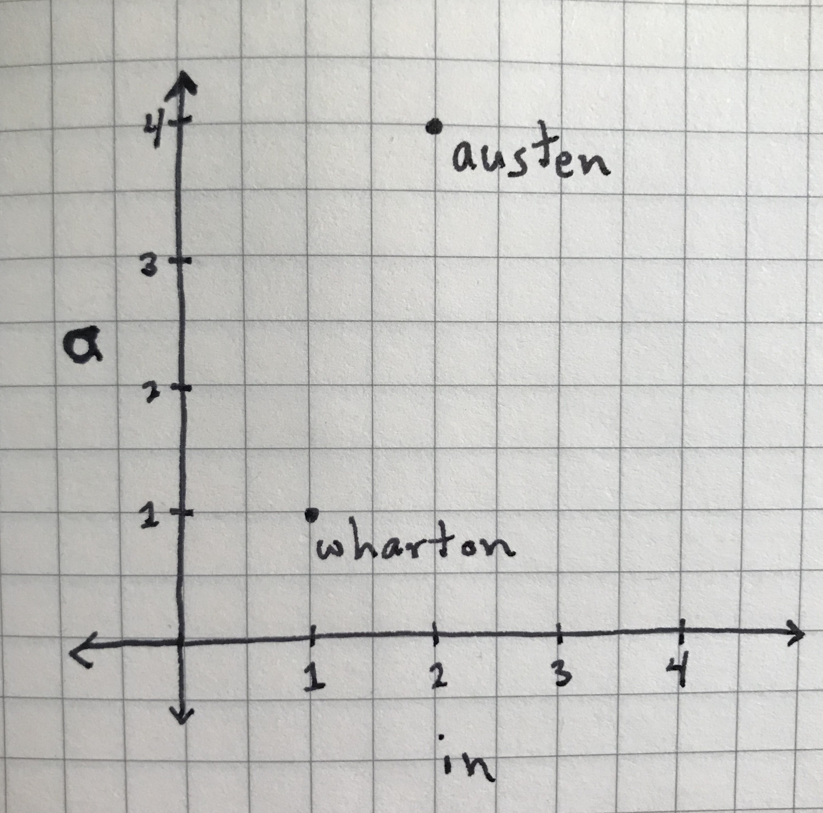
‘austen’ and ‘wharton’ samples represented as data points.
On this graph, the austen and wharton samples are each represented as data points along two axes, or dimensions. The horizontal x-axis represents the values for the word “in” and the vertical y-axis represents the values for the word “a.” Though it may look simple, this representation allows us to imagine a spatial relationship between data points based on their features, and this spatial relationship, what we’re calling similarity or distance, can tell you something about which samples are alike.
Here’s where it gets cool. You can represent two features as two dimensions and visualize your samples using the Cartesian coordinate system. Naturally you could also visualize our samples in three dimensions if you had three features. If you had four or more features, you couldn’t visualize the samples anymore: for how could you create a four-dimensional graph? But it doesn’t matter, because no matter how many features or dimensions you have, you can still calculate distance in the same way. If you’re working with word frequencies, as we are here, you can have as many features/dimensions as you do words in a text. For the rest of this lesson, the examples of distance measures will use two dimensions, but when you calculate distance with Python later in this tutorial, you’ll calculate over thousands of dimensions using the same equations.
Distance and Similarity
Now you’ve taken your samples and rendered them as points in space. As a way of understanding how these two points are related to each other, you might ask: How far apart or close together are these two points? The answer to “How far apart are these points?” is their distance and the answer to “How close together are these points?” is their similarity. In addition to this distinction, similarity, as I mentioned previously, can refer to a larger category of similarity measures, whereas distance usually refers to a more narrow category that measures difference in Cartesian space.
It may seem redundant or confusing to use both terms, but in text analysis these concepts are usually reciprocally related (i.e., distance is merely the opposite of similarity and vice versa). I bring them both up for a simple reason: out in the world you are likely to encounter both terms, sometimes used more or less interchangeably. When you are measuring by distance, the most closely related points will have the lowest distance, but when you are measuring by similarity, the most closely related points will have the highest similarity. For the most part you will encounter distance rather than similarity, but this explanation may come in handy if you encounter a program or algorithm that outputs similarity instead. We will revisit this distinction in the Cosine Similarity and Cosine Distance section.
You might think that calculating distance is as simple as drawing a line between these two points and calculating its length. And it can be! But in fact there are many ways to calculate the distance between two points in Cartesian space, and different distance measures are useful for different purposes. For instance, the SciPy pdist function that you’ll use later on lists 22 distinct measures for distance. In this tutorial, you’ll learn about three of the most common distance measures: city block distance, Euclidean distance, and cosine distance.
Three Types of Distance/Similarity
City Block (Manhattan) Distance
The simplest way of calculating the distance between two points is, perhaps surprisingly, not to go in a straight line, but to go horizontally and then vertically until you get from one point to the other. This is simpler because it only requires you to subtract rather than do more complicated calculations.
For example, your wharton sample is at point (1,1): its x-coordinate is 1 (its value for “in”), and its y-coordinate is 1 (its value for “a”). Your austen sample is at point (2,4): its x-coordinate is 2, and its y-coordinate is 4. We want to calculate distance by looking at the differences between the x- and y-coordinates. The dotted line in the following graph shows what you’re measuring:
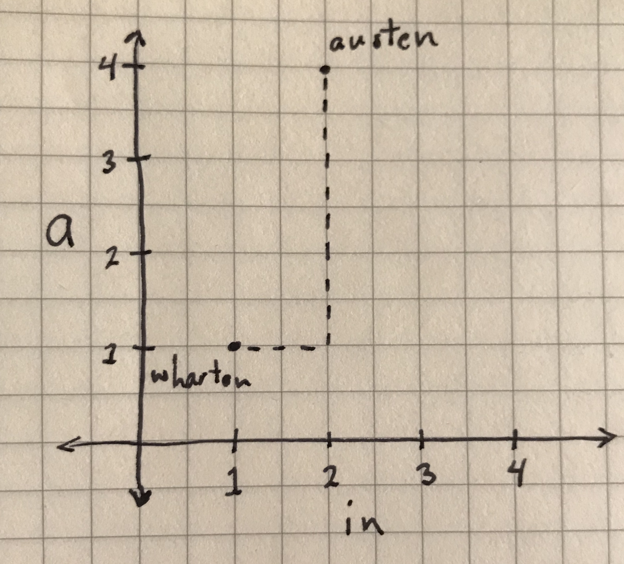
The distance between ‘austen’ and ‘wharton’ points by ‘city block’ distance.
You can see here why it’s called city block distance, or “Manhattan distance” if you prefer a more New York-centric pun. “Block” refers to the grid-like layout of North American city streets, especially those found in New York City. The graphs of city block distance, like the previous one, resemble those grid layouts. On this graph it’s easy to tell that the length of the horizontal line is 1 and the length of the vertical line is 3, which means the city block distance is 4. But how would you abstract this measure? As I alluded to above, city block distance is the sum of the differences between the x- and y-coordinates. So for two points with any values (let’s call them \((x_1, y_1)\) and \((x_2, y_2)\)), the city block distance is calculated using the following expression:
\[|x_2 - x_1| + |y_2 - y_1|\](The vertical bars you see are for absolute value; they ensure that even if \(x_1\) is greater than \(x_2\), your values are still positive.) Try it out with your two points (1,1) and (2,4):
\[|2 - 1| + |4 - 1| = |1| + |3| = 1 + 3 = 4\]And that’s it! You could add a third coordinate, call it “z,” or as many additional dimensions as you like for each point, and still calculate city block distance fairly easily. Because city block distance is easy to understand and calculate, it’s a good one to start with as you learn the general principles. But it’s less useful for text analysis than the other two distance measures we’re covering. And in most cases, you’re likely to get better results using the next distance measure, Euclidean distance.
Euclidean Distance
At this point I can imagine what you’re thinking: Why should you care about “going around the block”? The shortest distance between two points is a straight line, after all.
Euclidean distance, named for the geometric system attributed to the Greek mathematician Euclid, will allow you to measure the straight line. Look at the graph again, but this time with a line directly between the two points:
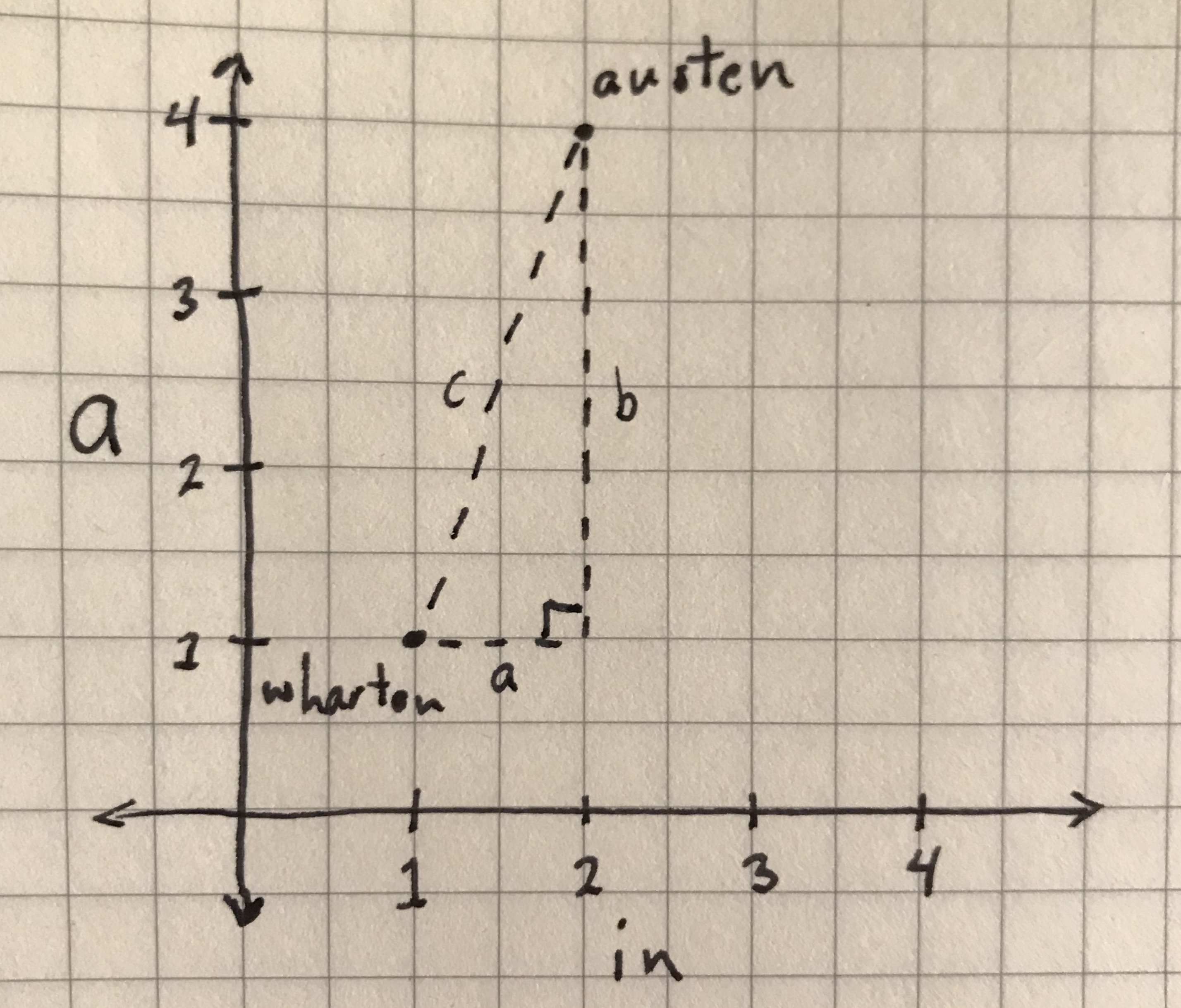
The distance between ‘austen’ and ‘wharton’ data points using Euclidean distance.
You’ll notice I left in the city block lines. If we want to measure the distance of the line (“c”) between our two points, you can think about that line as the hypotenuse of a right triangle, where the other two sides (“a” and “b”) are the city block lines from our last distance measurement.
You calculate the length of the line “c” in terms of “a” and “b” using the Pythagorean theorem:
\[a^2 + b^2 = c^2\]or:
\[c = \sqrt[]{a^2 + b^2}\]We know that the values of a and b are the differences between x- and y-coordinates, so the full formula for Euclidean distance can be written as the following expression:
\[\sqrt[]{(x_2 - x_1)^2 + (y_2 - y_1)^2}\]If you put the austen and wharton points into this formula, you get:
\(\sqrt[]{(2 - 1)^2 + (4 - 1)^2} = \sqrt[]{1^2 + 3^2} = \sqrt[]{1 + 9} = \sqrt[]{10} = 3.16\)1
The Euclidean distance result is, as you might expect, a little less than the city block distance. Each measure tells you something about how the two points are related, but each also tells you something different about that relationship because what “distance” means for each measure is different. One isn’t inherently better than the other, but it’s important to know that distance isn’t a set fact: the distance between two points can be quite different depending on how you define distance in the first place.
Cosine Similarity and Cosine Distance
To emphasize this point, the final similarity/distance measure in this lesson, cosine similarity, is very different from the other two. This measure is more concerned with the orientation of the two points in space than it is with their exact distance from one another.
If you draw a line from the origin—the point on the graph at the coordinates (0, 0)—to each point, you can identify an angle, \(\theta\), between the two points, as in the following graph:
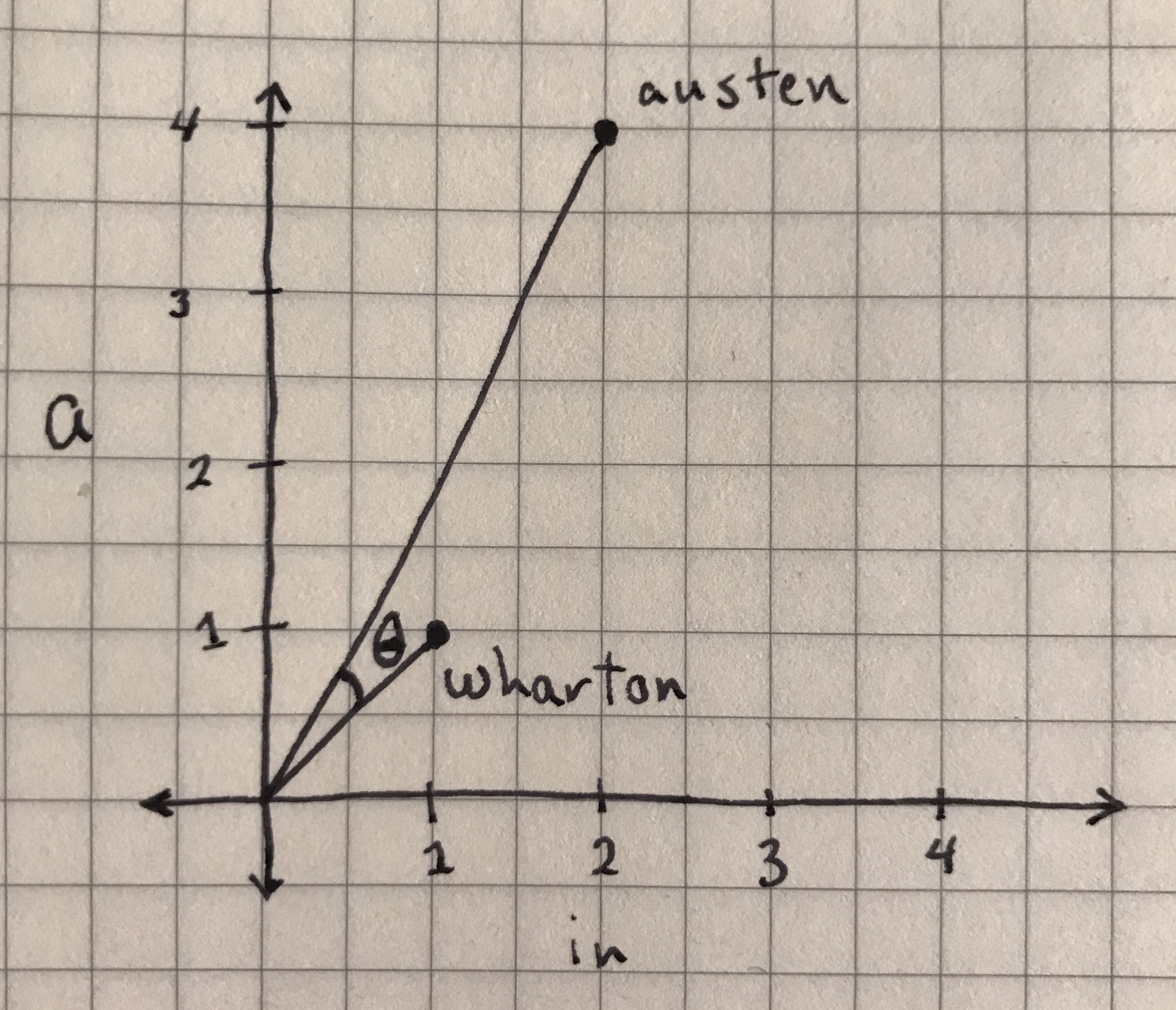
The angle between the ‘austen’ and ‘wharton’ data points, from which you will take the cosine.
The cosine similarity between the two points is simply the cosine of this angle. Cosine is a trigonometric function that, in this case, helps you describe the orientation of two points. If two points were 90 degrees apart, that is if they were on the x-axis and y-axis of this graph as far away from each other as they can be in this graph quadrant, their cosine similarity would be zero, because \(cos(90) = 0\). If two points were 0 degrees apart, that is if they existed along the same line, their cosine similarity would 1, because \(cos(0) = 1\).
Cosine provides you with a ready-made scale for similarity. Points that have the same orientation have a similarity of 1, the highest possible. Points that have 90 degree orientations have a similarity of 0, the lowest possible.2 Any other value will be somewhere in between.
You needn’t worry very much about how to calculate cosine similarity algebraically. Any programming environment will calculate it for you. But it’s possible to determine the cosine similarity by beginning only with the coordinates of two points, \((x_1, y_1)\) and \((x_2, y_2)\):
\[cos(\theta) = (x_1x_2 + y_1y_2)/(\sqrt[]{x_1^2 + y_1^2}\sqrt[]{x_2^2 + y_2^2})\]If you enter in your two austen and wharton coordinates, you get:
\((1\times2 + 1\times4)/(\sqrt[]{1^2 + 1^2}\sqrt[]{2^2 + 4^2}) = 6/(\sqrt[]{2}\sqrt[]{20}) = 6/6.32 = 0.95\)3
The cosine similarity of our austen sample to our wharton sample is quite high, almost 1. The result is borne out by looking at the graph, on which we can see that the angle \(\theta\) is fairly small. Because the two points are closely oriented, their cosine similarity is high. To put it another way: according to the measures you’ve seen so far, these two texts are pretty similar to one another.
But note that you’re dealing with similarity here and not distance. The highest value, 1, is reserved for the two points that are most close together, while the lowest value, 0, is reserved for the two points that are the least close together. This is the exact opposite of Euclidean distance, in which the lowest values describe the points closest together. To remedy this confusion, most programming environments calculate cosine distance by simply subtracting the cosine similarity from one. So cosine distance is simply \(1 - cos(\theta)\). In your example, the cosine distance would be:
\[1 - 0.95 = 0.05\]This low cosine distance is more easily comparable to the Euclidean distance you calculated previously, but it tells you the same thing as the cosine similarity result: that the austen and wharton samples, when represented only by the number of times they each use the words “a” and “in,” are fairly similar to one another.
How To Know Which Distance Measure To Use
These measures aren’t at all the same thing, and they yield quite different results. Yet they’re all types of distance, ways of describing the relationship between two data samples. This distinction illustrates the fact that, even at a very basic level, the decisions you make as an investigator can have an outsized effect on your results.
In this case, the question you must ask is: How do I measure the relationship between two points? The answer to that question depends on the nature of the data you start with and what you’re trying to find out.
As you saw in the previous section, city block distance and Euclidean distance are similar because they are both concerned with the lengths of lines between two points. This fact makes them more interchangeable. In most cases, Euclidean distance will be preferable over city block because it is more direct in its measurement of a straight line between two points.
Cosine distance is another story. The choice between Euclidean and cosine distance is an important one, especially when working with data derived from texts. I’ve already illustrated that cosine distance is only concerned with the orientation of two points and not with their exact placement. This means that cosine distance is much less effected by magnitude, or how large your numbers are.
To illustrate this, say for example that your points are (1,2) and (2,4) (instead of the (1,1) and (2,4) you used in the last section). The internal relationship within the two sets of coordinates is the same: a ratio of 1:2. But the points aren’t identical: the second set of coordinates has twice the magnitude of the first.
The Euclidean distance between these two points is:
\[\sqrt[]{(2 - 1)^2 + (4 - 2)^2} = \sqrt[]{1^2 + 2^2} = \sqrt[]{1 + 4} = \sqrt[]{5} = 2.24\]But their cosine similarity is:
\[(1\times2 + 2\times4)/(\sqrt[]{1^2 + 2^2}\sqrt[]{2^2 + 4^2}) = 10/(\sqrt[]{5}\sqrt[]{20}) = 10/\sqrt[]{100} = 10/10 = 1\]So their cosine distance is:
\[1 - 1 = 0\]Where Euclidean distance is concerned, these points are only a little distant from one another. While in terms of cosine distance, these two points are not at all distant. This is because Euclidean distance accounts for magnitude while cosine distance does not. Another way of putting this is that cosine distance measures whether the relationship among your various features is the same, regardless of how much of any one thing is present. This fact would be true if one of your points was (1,2) and the other was (300,600) as well.
Cosine distance is sometimes very good for text-related data. Often texts are of very different lengths. If words have vastly different counts but exist in the text in roughly the same proportion, cosine distance won’t worry about the raw counts, only their proportional relationships to each other. Otherwise, as with Euclidean distance you might wind up saying something like, “All the long texts are similar, and all the short texts are similar.” With text, it’s often better to use the distance measure that disregards differences in magnitude and focuses on the proportions of features.
However, if you know your sample texts are all roughly the same size (or if you have subdivided all your texts into equally-sized “chunks,” a common pre-processing step), you might prefer to account for relatively small differences in magnitude by using Euclidean distance. For non-text data where the size of the sample is unlikely to effect the features, Euclidean distance is sometimes preferred.
There’s no one answer for which distance measure to choose. As you’ve learned, it’s highly dependent on your data and your research question. That’s why it’s important to know your data well before you start out. If you’re stacking other methods—like clustering or a machine learning algorithm—on top of distance measures, you’ll certainly want to understand the distinction between distance measures and how choosing one over the other may effect your results down the line.
Calculating Distance in Python
Now that you understand city block, Euclidean, and cosine distance, you’re ready to calculate these measures using Python. For your example data, you’ll use the plain text files of EarlyPrint texts published in 1666, and the metadata for those files that you downloaded earlier. First, unzip the text files and place the 1666_texts/ directory inside your working folder (i.e. The directory 1666_texts/ file will need to be in the same folder as similarity.py for this to work).
Counting Words
To begin, you’ll need to import the libraries (Pandas, SciPy, and scikit-learn) that you installed in the Setup and Installation section , as well as a built-in library called glob.
Create a new blank file in your text editor of choice and name it similarity.py. (You can also download my complete version of this script.) At the top of the file, type:
import glob
import pandas as pd
from sklearn.feature_extraction.text import CountVectorizer
from scipy.spatial.distance import pdist, squareform
The scikit-learn and SciPy libraries are both very large, so the from _____ import _____ syntax allows you to import only the functions you need.
From this point, scikit-learn’s CountVectorizer class will handle a lot of the work for you, including opening and reading the text files and counting all the words in each text. You’ll first create an instance of the CountVectorizer class with all of the parameters you choose, and then run that model on your texts.
Scikit-learn gives you many parameters to work with, but you’ll need three:
-
Set
inputto"filename"to tellCountVectorizerto accept a list of filenames to open and read. -
Set
max_featuresto1000to capture only the 1000 most frequent words. Otherwise, you’ll wind up with hundreds of thousands of features that will make your calculations slower without adding very much additional accuracy. -
Set
max_dfto0.7. DF stands for document frequency. This parameter tellsCountVectorizerthat you’d like to eliminate words that appear in more than 70% of the documents in the corpus. This setting will eliminate the most common words (articles, pronouns, prepositions, etc.) without the need for a stop words list.
You can use the glob library you imported to create the list of file names that CountVectorizer needs. To set the three scikit-learn parameters and run CountVectorizer, type:
# Use the glob library to create a list of file names
filenames = glob.glob("1666_texts/*.txt")
# Parse those filenames to create a list of file keys (ID numbers)
# You'll use these later on.
filekeys = [f.split('/')[-1].split('.')[0] for f in filenames]

# Create a CountVectorizer instance with the parameters you need
vectorizer = CountVectorizer(input="filename", max_features=1000, max_df=0.7)
# Run the vectorizer on your list of filenames to create your wordcounts
# Use the toarray() function so that SciPy will accept the results
wordcounts = vectorizer.fit_transform(filenames).toarray()
And that’s it! You’ve now counted every word in all 142 texts in the test corpus. To interpret the results, you’ll also need to open the metadata file as a Pandas DataFrame. Add the following to the next line of your file:
metadata = pd.read_csv("1666_metadata.csv", index_col="TCP ID")
Adding the index_col="TCP ID" setting will ensure that the index labels for your metadata table are the same as the file keys you saved above. Now you’re ready to begin calculating distances.
Calculating Distance using SciPy
Calculating distance in SciPy comprises two steps: first you calculate the distances, and then you must expand the results into a squareform matrix so that they’re easier to read and process. It’s called squareform because the columns and rows are the same, so the matrix is symmetrical, or square.4 The distance function in SciPy is called pdist and the squareform function is called squareform. Euclidean distance is the default output of pdist, so you’ll use that one first. To calculate distances, call the pdist function on your DataFrame by typing pdist(wordcounts). To get the squareform results, you can wrap that entire call in the squareform function: squareform(pdist(wordcounts)). To make this more readable, you’ll want to put it all into a Pandas DataFrame. On the next line of your file, type:
euclidean_distances = pd.DataFrame(squareform(pdist(wordcounts)), index=filekeys, columns=filekeys)
print(euclidean_distances)
You need to declare that the index variable for the rows and the column variable will both refer back to the filekeys you saved when you originally read the files. Stop now, save this file, and run it from the command line by navigating to the appropriate directory in your Terminal application and typing python3 similarity.py. The script will print a matrix of the Euclidean distances between every text in the dataset!
In this “matrix,” which is really just a table of numbers, the rows and columns are the same. Each row represents a single EarlyPrint document, and the columns represent the exact same documents. The value in every cell is the distance between the text from that row and the text from that column. This configuration creates a diagonal line of zeroes through the center of your matrix: where every text is compared to itself, the distance value is zero.
EarlyPrint documents are corrected and annotated versions of documents from the Early English Books Online–Text Creation Partnership, which includes a document for almost every book printed in England between 1473 and 1700. This sample dataset includes all the texts published in 1666—the ones that are currently publicly available (the rest will be available after January 2021). What your matrix is showing you, then, is the relationships among books printed in England in 1666. This includes texts from a variety of different genres on all sorts of topics: religious texts, political treatises, and literary works, to name a few. One thing a researcher might want to know right away with a text corpus as thematically diverse as this one is: Is there a computational way to determine the kinds of similarity that a reader cares about? When you calculate the distances among such a wide variety of texts, will the results “make sense” to an expert reader? You’ll try to answer these questions in the exercise that follows.
There’s a lot you could do with this table of distances beyond the kind of sorting illustrated in this example. You could use it as an input for an unsupervised clustering of the texts into groups, and you could employ the same measures to drive a machine learning model. If you wanted to understand these results better, you could create a heatmap of this table itself, either in Python or by exporting this table as a CSV and visualizing it elsewhere.
As an example, let’s take a look at the five texts that are the most similar to Robert Boyle’s Hydrostatical paradoxes made out by new experiments, which is part of this dataset under the ID number A28989. The book is a scientific treatise and one of two works Boyle published in 1666. By comparing distances, you could potentially find books that are either thematically or structurally similar to Boyle’s: either scientific texts (rather than religious works, for instance) or texts that have similar prose sections (rather than poetry collections or plays, for instance).
Let’s see what texts are similar to Boyle’s book according to their Euclidean distance. You can do this using Pandas’s nsmallest function. In your working file, remove the line that says print(euclidean_distances), and in its place type:
top5_euclidean = euclidean_distances.nsmallest(6, 'A28989')['A28989'][1:]
print(top5_euclidean)
Why six instead of five? Because this is a symmetrical or square matrix, one of the possible results is always the same text. Since we know that any text’s distance to itself is zero, it will certainly come up in our results. We need five more in addition to that one, so six total. But you can use the slicing notation [1:] to remove that first redundant text.
The results you get should look like the following:
A62436     988.557029
A43020     988.622274
A29017    1000.024000
A56390    1005.630151
A44061    1012.873141
Your results will contain only the Text Creation Partnership ID numbers, but you can use the metadata DataFrame you created earlier to get more information about the texts. To do so, you’ll use the .loc method in Pandas to select the rows and columns of the metadata that you need. On the next line of your file, type:
print(metadata.loc[top5_euclidean.index, ['Author','Title','Keywords']])
In this step, you’re telling Pandas to limit the rows to the file keys in your Euclidean distance results and limit the columns to author, title, and subject keywords, as in the following table:5
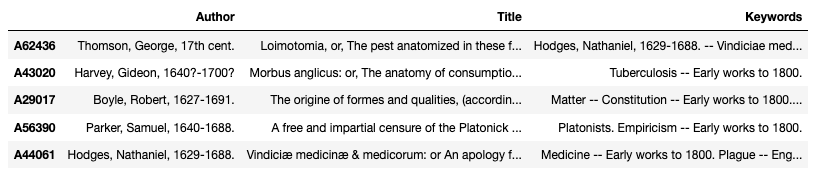
Metadata for the top five similar texts by Euclidean distance.
There’s some initial success on this list, suggesting that our features are successfully finding texts that a human would recognize as similar. The first two texts, George Thomson’s work on plague and Gideon Harvey’s on tuberculosis, are both recognizably scientific and clearly related to Boyle’s. But the next one is the other text written by Boyle, which you might expect to come up before the other two. The next question to ask is: what different results might you get with cosine distance?
You can calculate cosine distance in exactly the way you calculated Euclidean distance, but with a parameter that specifies the type of distance you want to use. On the next lines of your file, type:
cosine_distances = pd.DataFrame(squareform(pdist(wordcounts, metric='cosine')), index=filekeys, columns=filekeys)

top5_cosine = cosine_distances.nsmallest(6, 'A28989')['A28989'][1:]
print(top5_cosine)
Running the script will now output the top five texts for both Euclidean distance and cosine distance. (You could calculate city block distance by using metric='cityblock', but the results are unlikely be substantially different from Euclidean distance.) The results for cosine distance should look like the following:
A29017    0.432181
A43020    0.616269
A62436    0.629395
A57484    0.633845
A60482    0.663113
Right away you’ll notice a big difference. Because cosine distances are scaled from 0 to 1 (see the Cosine Similarity and Cosine Distance section for an explanation of why this is the case), we can tell not only what the closest samples are, but how close they are.6 Only one of the closest five texts has a cosine distance less than 0.5, which means most of them aren’t that close to Boyle’s text. This observation is helpful to know and puts some of the previous results into context. We’re dealing with an artificially limited corpus of texts published in just a single year; if we had a larger set, it’s likely we’d find texts more similar to Boyle’s.
You can now print the metadata for these results in the same way as in the previous example:
print(metadata.loc[top5_cosine.index, ['Author','Title','Keywords']])
The following table shows the metadata for the texts that cosine distance identified:
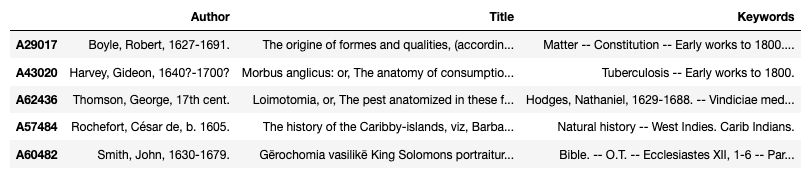
Metadata for the top five similar texts by cosine distance.
The first three texts in the list are the same as before, but their order has reversed. Boyle’s other text, as we might expect, is now at the top of the rankings. And as we saw in the numerical results, its cosine distance suggests it’s more similar than the next text down in this list, Harvey’s. The order in this example suggests that perhaps Euclidean distance was picking up on a similarity between Thomson and Boyle that had more to do with magnitude (i.e. the texts were similar lengths) than it did with their contents (i.e. words used in similar proportions). The final two texts in this list, though it is hard to tell from their titles, are also fairly relevant to Boyle’s. Both of them deal with topics that were part of early modern scientific thought, natural history and aging, respectively. As you might expect, because cosine distance is more focused on comparing the proportions of features within individual samples, its results were slightly better for this text corpus. But Euclidean distance was on the right track, even if it didn’t capture all the similarity you were looking for. If as a next step you expanded these lists out to ten texts, you’d likely see even more differences between results for the two distance measures.
It’s crucial to note that this exploratory investigation into text similarity didn’t give you a lot of definitive answers. Instead it raises many interesting questions: Which words (features) caused these specific books (samples) to manifest as similar to one another? What does it mean to say that two texts are “similar” according to raw word counts rather than some other feature set? What else can we learn about the texts that appeared in proximity to Boyle’s? Like many computational methods, distance measures provide you with a way to ask new and interesting questions of your data, and initial results like these can lead you down new research paths.
Next Steps
I hope this tutorial gave you a more concrete understanding of basic distance measures as well as a handle on when to choose one over the other. As a next step, and for better results in assessing similarity among texts by their words, you might consider using TF-IDF (Term Frequency–Inverse Document Frequency) instead of raw word counts. TF-IDF is a weighting system that assigns a value to every word in a text based on the relationship between the number of times a word appears in that text (its term frequency) and the number of texts it appears in through the whole corpus (its document frequency). This method is often used as an initial heuristic for a word’s distinctiveness and can give the researcher more information than a simple word count. To understand exactly what TF-IDF is and what calculating it entails, see Matthew J. Lavin’s Analyzing Documents with TF-IDF. You could take TF-IDF results you made using Lavin’s procedure and replace the matrix of word counts in this lesson.
In the future you may use distance measures to look at the most similar samples in a large data set as you did in this lesson. But it’s even more likely that you’ll encounter distance measures as a near-invisible part of a larger data mining or text analysis approach. For example, k-means clustering uses Euclidean distance by default to determine groups or clusters in a large dataset. Understanding the pros and cons of distance measures could help you to better understand and use a method like k-means clustering. Or perhaps more importantly, a good foundation in understanding distance measures might help you to assess and evaluate someone else’s digital work more accurately.
Distance measures are a good first step to investigating your data, but a choice between the three different metrics described in this lesson—or the many other available distance measures—is never neutral. Understanding the advantages and trade-offs of each can make you a more insightful researcher and help you better understand your data.
-
I rounded this result to the nearest hundredth place to make it more readable. ↩
-
A similarity lower than 0 is indeed possible. If you move to another quadrant of the graph, two points could have a 180 degree orientation, and then their cosine similarity would be -1. But because you can’t have negative word counts (our basis for this entire exercise), you’ll never have a point outside this quadrant. ↩
-
Once again, I’ve done some rounding in the final two steps to make this operation more readable. ↩
-
SciPy’s
pdistfunction outputs what’s called a “sparse matrix” to save space and processing power. This output is fine if you’re using this as part of a pipeline for another purpose, but we want the “squareform” matrix so that we can see all the results. ↩ -
I made these results a little easier to read by running identical code in a Jupyter Notebook. If you run the code on the command line, the results will be the same, but they will be formatted a little differently. ↩
-
It’s certainly possible to scale the results of Euclidean or city block distance as well, but it’s not done by default. ↩