Contents
- Assumptions
- Lesson Goals
- Introduction
- An Example of dplyr in Action
- Pipe Operator
- We Need a New Dataset
- What is Dplyr?
- Putting it All Together
- Conclusion
Assumptions
This lesson makes a few assumptions about your understanding of R. If you have not completed the R Basics with Tabular Data lesson, I suggest you complete that first. Having a background in another programming language will also be beneficial. If you need a place to start, I recommend working through the Programming Historian’s excellent Python tutorials.
Lesson Goals
By the end of this lesson, you will:
- Know how to organize data to be “tidy” and why this is important.
- Understand the dplyr package and use it to manipulate and wrangle with data.
- Become acquainted with the pipe operator in R and observe how it can assist you in creating more readable code.
- Learn to work through some basic examples of data manipulation to gain a foundation in exploratory data analysis.
Introduction
Data you find “in the wild” will rarely be in a format necessary for analysis, and you will need to manipulate it before exploring the questions you are interested in. This may take more time than doing the analysis itself! In this tutorial, we will learn some basic techniques for manipulating, managing, and wrangling with our data in R. Specifically, we will rely on the philosophy of “tidy data” as articulated by Hadley Wickham.
According to Wickham, data is “tidy” when it meets three key criteria:
- Each observation is in a row.
- Each variable is in a column.
- Each value has its own cell.
Being observant of these criteria allows us to recognize when data is organized or unorganized. It also provides us a standardized schema and set of tools for cleaning up some of the most common ways that datasets are “messy:”
- Column headers are values, not variable names.
- Multiple variables are stored in one column.
- Variables are stored in both rows and columns.
- Multiple types of observational units are stored in the same table.
- A single observational unit is stored in multiple tables.
Perhaps most importantly, keeping our data in this format allows us to use a collection of packages in the “tidyverse,” which are designed to specifically work with tidy data. By making sure that our input and output are tidy, we only have to use a small set of tools to solve a large number of questions. In addition, we can combine, manipulate, and split tidy datasets as we see fit.
In this tutorial, we will be focusing on the dplyr package of the tidyverse, but it is worth briefly mentioning some others we will be running into:
magittr–This package gives us access to the forward pipe operator and makes our code easier to read. ggplot2–This package utilizes the “Grammar of Graphics” to provide an easy way to visualize our data. readr–This package makes available a faster and more streamlined method of importing rectangular data, such as csv files. tibble–This package provides us access to a reconceptualization of data frames that are easier to work with and print.
If you have not already done so, you should install and load the “tidyverse” before beginning. In addition, make sure that you have the latest version of R and the latest version of R Studio installed for your respective platform.
Copy the following code into RStudio. To run it, you need to highlight the lines and press Ctrl+Enter (Command+Enter on Mac OS):
# Install tidyverse libraries and load it
# Do not worry if this takes a while

install.packages("tidyverse")
library(tidyverse)
An Example of dplyr in Action
Let’s go through an example to see how dplyr can aid us as historians by inputting U.S. decennial census data from 1790 to 2010. Download the data by clicking here and place it in the folder that you will use to work through the examples in this tutorial.
Since the data is in a csv file, we are going to use the read_csv() command in tidyverse’s readr package.
The read_csv function takes the path of a file we want to import from as a variable so make sure that you have it set up correctly.
# Import CSV File and save to us_state_populations_import
# Make sure you set the path of the file correctly
us_state_populations_import<-read_csv("introductory_state_example.csv")
After you import the data, you will notice that there are three columns: one for the population, one for the year, and one for the state. This data is already in a tidy format providing us a multitude of options for further exploration.
For this example, let’s visualize the population growth of California and New York to gain a better understanding of Western migration. We will use dplyr to filter our data so that it only contains information about the states we are interested in, and we will use ggplot2 to visualize this information. This exercise is just to provide you a taste of what dplyr can do, so don’t worry if you don’t understand the code at this time.
# Filter to California and New York states only
california_and_new_york_state_populations<-us_state_populations_import %>%
  filter(state %in% c("California", "New York"))

# Plot California and New York State Populations
ggplot(data=california_and_new_york_state_populations, aes(x=year, y=population, color=state)) +
  geom_line() +
  geom_point()
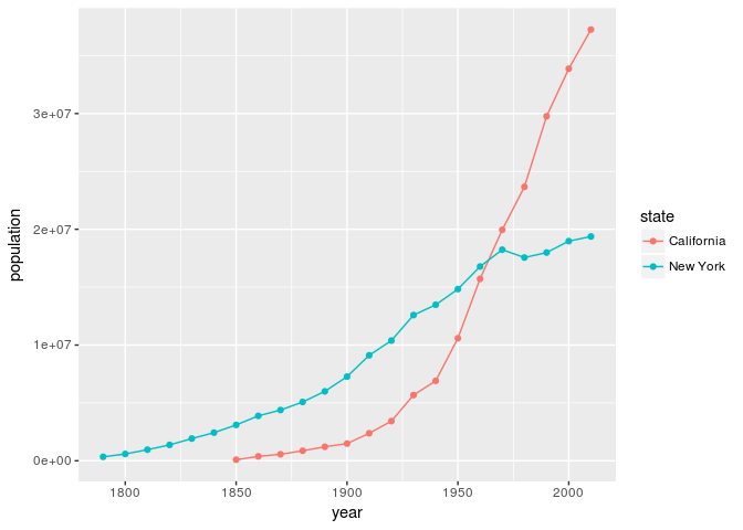
Graph of California and New York population
As we can see, the population of California has grown considerably compared to New York. While this particular example may seem obvious given the history of U.S. migration, the code itself provides us a foundation that we can build on to ask a multitude of similar questions. For instance, with a quick change of code, we can create a similar graph with two different states such as Mississippi and Virginia.
# Filter to Mississippi and Virginia
mississippi_and_virginia_state_populations<-us_state_populations_import %>%
  filter(state %in% c("Mississippi", "Virginia"))

# Plot California and New York State Populations
ggplot(data=mississippi_and_virginia_state_populations, aes(x=year, y=population, color=state)) +
  geom_line() +
  geom_point()
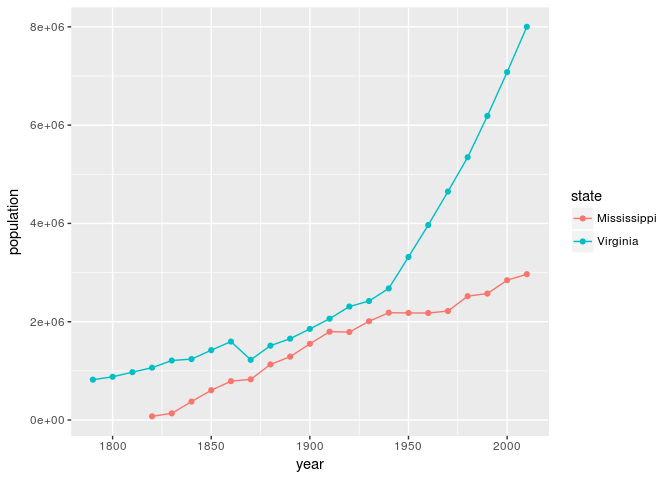
Graph of Mississippi and Virginia population
Quickly making changes to our code and reanalyzing our data is a fundamental part of exploratory data analysis (EDA). Rather than trying to “prove” a hypothesis, exploratory data analysis helps us understand our data better and ask questions about it. For historians, EDA provides an easy means of knowing when to dig deeper into a subject and when to step back, and it is an area where R excels.
Pipe Operator
Before looking at dplyr, we need to go over the pipe operator (%>%) in R since we will often run into it in our examples. As mentioned earlier, the pipe operator is part of the magrittr package created by Stefan Milton Bache and Hadley Wickham and is included in the tidyverse. Its name is an homage to surrealest painter Rene Magritte, whose “The Treachery of Images” famously depicted a pipe with the words “this is not a pipe” underneath in French.
The pipe operator allows you to pass what is to the left of the pipe as the first variable in a function specified on the right. Although it may seem strange at first, once you learn it, you will find that it makes your code more readable by avoiding nested statements. Don’t worry if all this is a little confusing right now. It will become more clear as we go through the examples.
Let’s say that we are interested in getting the square root of each population value and then summing all the square roots before getting the mean. Obviously, this isn’t a useful measurement, but it demonstrates just how quickly R code can become difficult to read. Normally, we would nest such statements:
mean(sum(sqrt(us_state_populations_import$population)))

## [1] 1256925
As you can see, with enough nested commands, it is hard to remember how many parenthesis you need and makes the code awkward to read. To mitigate this, some people may create temporary vectors in between each function call.
# Get square root of all the state populations

sqrt_state_populations_vector<-sqrt(us_state_populations_import$population)

# Get sum of all the sqrts of the temporary variable

sum_sqrt_state_populations_vector<-sum(sqrt_state_populations_vector)

# Get mean of the temporary variable

mean_sum_sqrt_state_populations_vector<-mean(sum_sqrt_state_populations_vector)

# Display the mean

mean_sum_sqrt_state_populations_vector

## [1] 1256925
Although you get the same answer, this is a lot more readable. However, it can quickly clutter your workspace if you forget to delete the temporary vectors. The pipe operator does all this for you. Here is the same code using the pipe operator.
us_state_populations_import$population%>%sqrt%>%sum%>%mean

## [1] 1256925
This is a lot easier to read, and you could make it even more clear by writing this on multiple lines.
# Make sure to put the operator at the end of the line
us_state_populations_import$population%>%
    sqrt%>%
    sum%>%
    mean

## [1] 1256925
Please note that the vectors or data frames that the pipe operator creates are discarded after the operation is complete. If you want to store them, you should pass them to a new variable.
permanent_sqrt_and_sum_state_populations_vector <- us_state_populations_import$population%>%sqrt%>%sum%>%mean
permanent_sqrt_and_sum_state_populations_vector

## [1] 1256925
We Need a New Dataset
Now that we have an understanding of the pipe operator, we are ready to begin looking at and wrangling with some data. Unfortunately, for historians, there are only a few easily available datasets–perhaps you can help change this by making yours available to the public! We are going to rely on the history data package created by Lincoln Mullen.
Lets go ahead and install and load the package:
# Install historydata package
install.packages("historydata")

# Load historydata package
library(historydata)
This packages contains samples of historical datasets–the earlier U.S. Census data sample was taken from this package. Throughout this tutorial, we are specifically going to work with the early_colleges dataset that contains data about colleges founded before 1848. Lets start by loading the data and view it.
# Make sure you have installed the historydata package and loaded it before this

data(early_colleges)
early_colleges

## # A tibble: 65 x 6
##    college                original_name         city          state
##    <chr>                  <chr>                 <chr>         <chr>
##  1 Harvard                <NA>                  Cambridge     MA
##  2 William and Mary       <NA>                  Williamsburg  VA
##  3 Yale                   <NA>                  New Haven     CT
##  4 Pennsylvania, Univ. of <NA>                  Philadelphia  PA
##  5 Princeton              College of New Jersey Princeton     NJ
##  6 Columbia               King's College        New York      NY
##  7 Brown                  <NA>                  Providence    RI
##  8 Rutgers                Queen's College       New Brunswick NJ
##  9 Dartmouth              <NA>                  Hanover       NH
## 10 Charleston, Coll. Of   <NA>                  Charleston    SC
##    established sponsorship
##          <int> <chr>
##  1        1636 Congregational; after 1805 Unitarian
##  2        1693 Anglican
##  3        1701 Congregational
##  4        1740 Nondenominational
##  5        1746 Presbyterian
##  6        1754 Anglican
##  7        1765 Baptist
##  8        1766 Dutch Reformed
##  9        1769 Congregational
## 10        1770 Anglican
## # ... with 55 more rows
As you can observe, this dataset contains the current name of the college, its original name, the city and state where it was founded, when the college was established, and its sponsorship. As we discussed earlier, before we can work with a dataset, it is important to think about how to organize the data. Let’s see if any of our data is not in a “tidy” format. Do you see any cells that do not match the three criteria for tidy data?
If you guessed the sponsorship of Harvard, you are correct. In addition to noting the original sponsorship, it also mentions that it changed sponsorship in 1805. Usually, you want to keep as much information about your data that you can, but for the purposes of this tutorial, we are going to change the column to only have the original sponsorship.
early_colleges[1,6] <- "Congregational"
early_colleges

## # A tibble: 65 x 6
##    college                original_name         city          state
##    <chr>                  <chr>                 <chr>         <chr>
##  1 Harvard                <NA>                  Cambridge     MA
##  2 William and Mary       <NA>                  Williamsburg  VA
##  3 Yale                   <NA>                  New Haven     CT
##  4 Pennsylvania, Univ. of <NA>                  Philadelphia  PA
##  5 Princeton              College of New Jersey Princeton     NJ
##  6 Columbia               King's College        New York      NY
##  7 Brown                  <NA>                  Providence    RI
##  8 Rutgers                Queen's College       New Brunswick NJ
##  9 Dartmouth              <NA>                  Hanover       NH
## 10 Charleston, Coll. Of   <NA>                  Charleston    SC
##    established sponsorship
##          <int> <chr>
##  1        1636 Congregational
##  2        1693 Anglican
##  3        1701 Congregational
##  4        1740 Nondenominational
##  5        1746 Presbyterian
##  6        1754 Anglican
##  7        1765 Baptist
##  8        1766 Dutch Reformed
##  9        1769 Congregational
## 10        1770 Anglican
## # ... with 55 more rows
Now that we have our data in a tidy format, we can shape it through the dplyr package.
What is Dplyr?
Dplyr is another part of the tidyverse that provides functions for manipulating and transforming your data. Because we are keeping our data “tidy,” we only need a small set of tools to explore our data. Compared to base R, using dplyr is often faster, and guarantees that if our input is tidy then our output will also be tidy. Perhaps most importantly, dplyr makes our code easier to read and utilizes “verbs” that are, in most cases, intuitive. Each function in dplyr corresponds to these verbs, with the five key ones being filter, select, arrange, mutate, and summarise–dplyr uses the British spelling. Let’s go through each of them individually to see how they work in practice.
Select
If we look at the early_colleges data, we can observe that there are a lot of NA’s in the original names column. NA signifies that the data is not available, and we may want to view our data with this column removed. dplyr’s select() function gives us the ability to do this. It takes the data frame you want to manipulate as the first argument, followed by a list signifying which columns you would like to keep:
# Remove the original names column using select()
# Note that you do not have to append the column name with a $ to the end of early_colleges since
# dplyr automatically assumes that a "," represents AND

select(early_colleges, college, city, state, established, sponsorship)

## # A tibble: 65 x 5
##    college                city          state established sponsorship
##    <chr>                  <chr>         <chr>       <int> <chr>
##  1 Harvard                Cambridge     MA           1636 Congregational
##  2 William and Mary       Williamsburg  VA           1693 Anglican
##  3 Yale                   New Haven     CT           1701 Congregational
##  4 Pennsylvania, Univ. of Philadelphia  PA           1740 Nondenominational
##  5 Princeton              Princeton     NJ           1746 Presbyterian
##  6 Columbia               New York      NY           1754 Anglican
##  7 Brown                  Providence    RI           1765 Baptist
##  8 Rutgers                New Brunswick NJ           1766 Dutch Reformed
##  9 Dartmouth              Hanover       NH           1769 Congregational
## 10 Charleston, Coll. Of   Charleston    SC           1770 Anglican
## # ... with 55 more rows
Let’s also go ahead and see how to write this using the pipe operator (%>%):
early_colleges%>%
    select(college, city, state, established, sponsorship)

## # A tibble: 65 x 5
##    college                city          state established sponsorship
##    <chr>                  <chr>         <chr>       <int> <chr>
##  1 Harvard                Cambridge     MA           1636 Congregational
##  2 William and Mary       Williamsburg  VA           1693 Anglican
##  3 Yale                   New Haven     CT           1701 Congregational
##  4 Pennsylvania, Univ. of Philadelphia  PA           1740 Nondenominational
##  5 Princeton              Princeton     NJ           1746 Presbyterian
##  6 Columbia               New York      NY           1754 Anglican
##  7 Brown                  Providence    RI           1765 Baptist
##  8 Rutgers                New Brunswick NJ           1766 Dutch Reformed
##  9 Dartmouth              Hanover       NH           1769 Congregational
## 10 Charleston, Coll. Of   Charleston    SC           1770 Anglican
## # ... with 55 more rows
Referencing each of the columns that we want to keep just to get rid of one is a little tedous. We can use the minus symbol (-) to demonstrate that we want to remove a column.
early_colleges%>%
    select(-original_name)

## # A tibble: 65 x 5
##    college                city          state established sponsorship
##    <chr>                  <chr>         <chr>       <int> <chr>
##  1 Harvard                Cambridge     MA           1636 Congregational
##  2 William and Mary       Williamsburg  VA           1693 Anglican
##  3 Yale                   New Haven     CT           1701 Congregational
##  4 Pennsylvania, Univ. of Philadelphia  PA           1740 Nondenominational
##  5 Princeton              Princeton     NJ           1746 Presbyterian
##  6 Columbia               New York      NY           1754 Anglican
##  7 Brown                  Providence    RI           1765 Baptist
##  8 Rutgers                New Brunswick NJ           1766 Dutch Reformed
##  9 Dartmouth              Hanover       NH           1769 Congregational
## 10 Charleston, Coll. Of   Charleston    SC           1770 Anglican
## # ... with 55 more rows
Filter
The filter() function does the same thing as the select function but rather than choosing the column name, we can use it to filter rows using a test requirement. For instance, we can view all the colleges that existed before the turn of the century.
early_colleges%>%
    filter(established < 1800)

## # A tibble: 20 x 6
##    college                  original_name         city           state
##    <chr>                    <chr>                 <chr>          <chr>
##  1 Harvard                  <NA>                  Cambridge      MA
##  2 William and Mary         <NA>                  Williamsburg   VA
##  3 Yale                     <NA>                  New Haven      CT
##  4 Pennsylvania, Univ. of   <NA>                  Philadelphia   PA
##  5 Princeton                College of New Jersey Princeton      NJ
##  6 Columbia                 King's College        New York       NY
##  7 Brown                    <NA>                  Providence     RI
##  8 Rutgers                  Queen's College       New Brunswick  NJ
##  9 Dartmouth                <NA>                  Hanover        NH
## 10 Charleston, Coll. Of     <NA>                  Charleston     SC
## 11 Hampden-Sydney           <NA>                  Hampden-Sydney VA
## 12 Transylvania             <NA>                  Lexington      KY
## 13 Georgia, Univ. of        <NA>                  Athens         GA
## 14 Georgetown               <NA>                  Washington     DC
## 15 North Carolina, Univ. of <NA>                  Chapel Hill    NC
## 16 Vermont, Univ. of        <NA>                  Burlington     VT
## 17 Williams                 <NA>                  Williamstown   MA
## 18 Tennessee, Univ. of      Blount College        Knoxville      TN
## 19 Union College            <NA>                  Schenectady    NY
## 20 Marietta                 <NA>                  Marietta       OH
##    established sponsorship
##          <int> <chr>
##  1        1636 Congregational
##  2        1693 Anglican
##  3        1701 Congregational
##  4        1740 Nondenominational
##  5        1746 Presbyterian
##  6        1754 Anglican
##  7        1765 Baptist
##  8        1766 Dutch Reformed
##  9        1769 Congregational
## 10        1770 Anglican
## 11        1775 Presbyterian
## 12        1780 Disciples of Christ
## 13        1785 Secular
## 14        1789 Roman Catholic
## 15        1789 Secular
## 16        1791 Nondenominational
## 17        1793 Congregational
## 18        1794 Secular
## 19        1795 Presbyterian with Congregational
## 20        1797 Congregational
Mutate
The mutate command allows you to add a column to your data frame. Right now, we have the city and state in two separate columns. We can use the paste command to combine two strings and specify a seperator. Let’s place them in a single column called “location.”
early_colleges%>%mutate(location=paste(city,state,sep=","))

## # A tibble: 65 x 7
##    college                original_name         city          state
##    <chr>                  <chr>                 <chr>         <chr>
##  1 Harvard                <NA>                  Cambridge     MA
##  2 William and Mary       <NA>                  Williamsburg  VA
##  3 Yale                   <NA>                  New Haven     CT
##  4 Pennsylvania, Univ. of <NA>                  Philadelphia  PA
##  5 Princeton              College of New Jersey Princeton     NJ
##  6 Columbia               King's College        New York      NY
##  7 Brown                  <NA>                  Providence    RI
##  8 Rutgers                Queen's College       New Brunswick NJ
##  9 Dartmouth              <NA>                  Hanover       NH
## 10 Charleston, Coll. Of   <NA>                  Charleston    SC
##    established sponsorship       location
##          <int> <chr>             <chr>
##  1        1636 Congregational    Cambridge,MA
##  2        1693 Anglican          Williamsburg,VA
##  3        1701 Congregational    New Haven,CT
##  4        1740 Nondenominational Philadelphia,PA
##  5        1746 Presbyterian      Princeton,NJ
##  6        1754 Anglican          New York,NY
##  7        1765 Baptist           Providence,RI
##  8        1766 Dutch Reformed    New Brunswick,NJ
##  9        1769 Congregational    Hanover,NH
## 10        1770 Anglican          Charleston,SC
## # ... with 55 more rows
Again, you need to remember that dplyr does not save the data or manipulate the original. Instead, it creates a temporary data frame at each step. If you want to keep it, you need to create a permanent variable.
early_colleges_with_location <- early_colleges%>%
    mutate(location=paste(city, state, sep=","))

# View the new tibble with the location added
early_colleges_with_location

## # A tibble: 65 x 7
##    college                original_name         city          state
##    <chr>                  <chr>                 <chr>         <chr>
##  1 Harvard                <NA>                  Cambridge     MA
##  2 William and Mary       <NA>                  Williamsburg  VA
##  3 Yale                   <NA>                  New Haven     CT
##  4 Pennsylvania, Univ. of <NA>                  Philadelphia  PA
##  5 Princeton              College of New Jersey Princeton     NJ
##  6 Columbia               King's College        New York      NY
##  7 Brown                  <NA>                  Providence    RI
##  8 Rutgers                Queen's College       New Brunswick NJ
##  9 Dartmouth              <NA>                  Hanover       NH
## 10 Charleston, Coll. Of   <NA>                  Charleston    SC
##    established sponsorship       location
##          <int> <chr>             <chr>
##  1        1636 Congregational    Cambridge,MA
##  2        1693 Anglican          Williamsburg,VA
##  3        1701 Congregational    New Haven,CT
##  4        1740 Nondenominational Philadelphia,PA
##  5        1746 Presbyterian      Princeton,NJ
##  6        1754 Anglican          New York,NY
##  7        1765 Baptist           Providence,RI
##  8        1766 Dutch Reformed    New Brunswick,NJ
##  9        1769 Congregational    Hanover,NH
## 10        1770 Anglican          Charleston,SC
## # ... with 55 more rows
Arrange
The arrange() function allows us to order our columns in a new way. Currently, the colleges are organized by year in ascending order. Lets place them in descending order of establishment, in this case, from the end of the Mexican-American War.
early_colleges %>%
    arrange(desc(established))

## # A tibble: 65 x 6
##    college               original_name city        state established
##    <chr>                 <chr>         <chr>       <chr>       <int>
##  1 Wisconsin, Univ. of   <NA>          Madison     WI           1848
##  2 Earlham               <NA>          Richmond    IN           1847
##  3 Beloit                <NA>          Beloit      WI           1846
##  4 Bucknell              <NA>          Lewisburg   PA           1846
##  5 Grinnell              <NA>          Grinnell    IA           1846
##  6 Mount Union           <NA>          Alliance    OH           1846
##  7 Louisiana, Univ. of   <NA>          New Orleans LA           1845
##  8 U.S. Naval Academy    <NA>          Annapolis   MD           1845
##  9 Mississipps, Univ. of <NA>          Oxford      MI           1844
## 10 Holy Cross            <NA>          Worchester  MA           1843
##    sponsorship
##    <chr>
##  1 Secular
##  2 Quaker
##  3 Congregational
##  4 Baptist
##  5 Congregational
##  6 Methodist
##  7 Secular
##  8 Secular
##  9 Secular
## 10 Roman Catholic
## # ... with 55 more rows
Summarise
The last key function in dplyr is summarise()–note the British spelling. Summarise() takes a function or operation, and is usually used to create a data frame that contains summary statistics for plotting. We will use it to calculate the average year that colleges before 1848 were founded.
early_colleges%>%summarise(mean(established))

## # A tibble: 1 x 1
##   `mean(established)`
##                 <dbl>
## 1            1809.831
Putting it All Together
Now that we have gone through the five main verbs for dplyr, we can use them to create a quick visualization of our data. Let’s go ahead and create a bar graph showing the number of secular and non-secular colleges founded before the U.S. War of 1812:
secular_colleges_before_1812<-early_colleges%>%
  filter(established < 1812)%>%
  mutate(is_secular=ifelse(sponsorship!="Secular", "no", "yes"))

ggplot(secular_colleges_before_1812) +
  geom_bar(aes(x=is_secular, fill=is_secular))+
  labs(x="Is the college secular?")
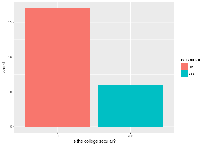
Number of secular and non-secular colleges before War of 1812
Again, by making a quick change to our code, we can also look at the number of secular versus non-secular colleges founded after the start of the War of 1812:
secular_colleges_after_1812<-early_colleges%>%
  filter(established > 1812)%>%
  mutate(is_secular=ifelse(sponsorship!="Secular", "no", "yes"))

ggplot(secular_colleges_after_1812) +
  geom_bar(aes(x=is_secular, fill=is_secular))+
  labs(x="Is the college secular?")
(
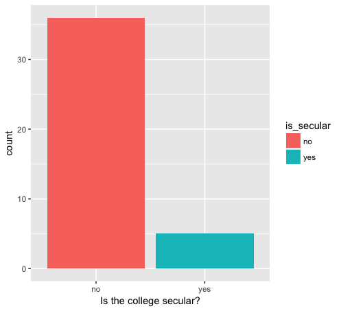
Number of secular and non-secular colleges after War of 1812
Conclusion
This tutorial should put you well on the way to thinking about how to organize and manipulate your data in R. Later, you will probably want to graph your data in some way. I recommend that you begin looking at the ggplot2 package for a set of tools that work well with dplyr. In addition, you may want to examine some of the other functions that come with dplyr to hone your skills. Either way, this should provide a good foundation to build on and cover a lot of the common problems you will encounter.